Practical B
Building a Numerical Integration Option Pricer in Excel
When an option payoff depends only on the spot rate at the maturity of the contract (e.g., European vanilla options) the price of the option can be calculated using the terminal spot distribution and the option payoff.
Task A: Set Up the Terminal Spot Distribution
Step 1: Set Up the Future Spots
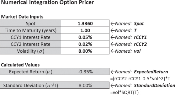
First, future spot levels must be generated using a log-normal distribution. The inputs to the function are:
- Spot (S): the current exchange rate in a given currency pair
- Interest rates (rCCY1 and rCCY2): continuously compounded risk-free interest rates in CCY1 and CCY2 of the currency pair
- Time to expiry (T): the time between the horizon date and expiry date measured in years
- Volatility (σ): the volatility of the spot log returns
Within log-normal world:

For a given return of X standard deviations:
This framework can be set up in an Excel sheet:

Under a normal distribution, a range from –5 to +5 standard deviations covers almost all possible theoretical returns. Starting with 0.1 steps, go from –5 to +5 standard deviations and calculate the return level and corresponding spot level for each standard deviation value:

Step 2: Calculate the Probability Density
The probability density function gives the relative likelihood of a random variable falling within a particular range of values. In Excel, =NORMSDIST(X) gives the cumulative normal distribution function, which is the probability of a normally distributed random variable with mean 0 and standard deviation 1 being at or below the input level X. Therefore, the probability of being between two levels (i.e., the probability density) can be calculated by taking the difference between two cumulative probabilities:


Note how the data in the rows is lined up; the probability density in a given row gives the probability of spot ending up between that spot level and the spot level in the row below.
The probability density can be plotted against spot to visualize the terminal spot distribution:

The implementation can be tested by changing the market data and observing how the terminal spot distribution changes. As explained in Chapter 5:
- Shorter maturity or lower volatility should lead to a tighter distribution.
- Longer maturity or higher volatility should lead to a wider distribution.
- Higher CCY2 interest rates or lower CCY1 interest rates should shift the distribution higher via the forward moving higher.
- Higher CCY1 interest rates or lower CCY2 interest rates should shift the distribution lower via the forward moving lower.
Task B: Set Up the Option Payoff and Calculate the Option Price
The option payoff can now be added into the framework. This numerical integration method can be used to price any payoff that only depends on spot at maturity, no matter how complicated, but the most obvious examples are:
- Long forward:

- Short forward:

- Vanilla call option: max(ST − K, 0)
- Vanilla put option: max(K − ST, 0)
Remember that these payoffs all return values in CCY2 per CCY1 (i.e., CCY2 pips) terms.
In Excel, add a new “option payoff” column and calculate the payoff at each spot level. To price a vanilla call option, the strike must be inputted:

Then the option payoff at maturity can be calculated at each spot level:

Within the numerical integration, multiply the probability of spot falling between two spot levels at maturity by the average payoff at maturity between two spot levels:


Probability-weighted option values are then summed to get the overall option value at maturity. The CCY2 pips option value must then be present valued (see Chapter 10) using the discount factor ![]() and converted into CCY1% by dividing by current spot:
and converted into CCY1% by dividing by current spot:

Testing
Finally, the pricer can be tested:
Test 1: A forward payoff struck at the forward should give (approximately) zero value:
-

Test 2: A vanilla CCY1 call option with S = K = 100, rCCY1 = rCCY2 = 0%, and T = 1.0 should have a value very slightly under 4.00 CCY1%:
-

