Constructing an ATM Curve in Excel

Within this practical, three methods of constructing an ATM curve are developed. First, an ATM curve is constructed using interpolation between market tenors. Then, an ATM curve is constructed using a parameterized model. Finally, weights are added to a simple ATM curve to demonstrate how ATM curves are maintained by traders in practice. These steps mirror the material developed in Chapter 11.

Task A: Constructing an ATM Curve Using Interpolation

When constructing an ATM curve based on market tenors, the expiry date for each market tenor must first be calculated using functions developed in Practical D. The ATM implied volatility is then manually inputted at each tenor. For the purposes of testing, a simple upward-sloping ATM curve can be used initially:

Using these inputs, a VBA function can interpolate to give the ATM volatility for any date. This function references the expiry dates and ATM volatilities at market tenors using named cells, with linear interpolation used to generate ATM volatility for expiry dates between tenors:

Function getATMVol(QueryDate As Long) As Double
    Dim Count As Long
    Dim TimeLow As Double, TimeHigh As Double
    Dim VolLow As Double, VolHigh As Double
    'Find the relevant Expiry date row (requires the Expiry dates
    to be ordered)
    Count = 1
    While Range("ExpiryDateRef").Offset(Count, 0) < QueryDate
    And Range("ExpiryDateRef").Offset(Count, 0) <> ""
        Count = Count + 1
    Wend
    If Range("ExpiryDateRef").Offset(Count, 0) = "" Then
        'Query Date beyond Maximum Expiry Date
        getATMVol = -1
    ElseIf Count = 1 And Range("ExpiryDateRef").Offset(Count, 0) >
    QueryDate Then
        'Query Date before Minimum Expiry Date
        getATMVol = -1
    ElseIf Range("ExpiryDateRef").Offset(Count, 0) = QueryDate Then
        'Exact Expiry Date Found
        getATMVol = Range("ATMVolRef").Offset(Count, 0)
    Else
        'Interpolate to get ATM Implied Volatility
        TimeLow = (Range("ExpiryDateRef").Offset(Count - 1, 0) -        Range("Horizon")) / 365
        TimeHigh = (Range("ExpiryDateRef").Offset(Count, 0) -        Range("Horizon")) / 365
        VolLow = Range("ATMVolRef").Offset(Count - 1, 0)
        VolHigh = Range("ATMVolRef").Offset(Count, 0)
        getATMVol = LinearVolatilityInterpolation(TimeLow, TimeHigh,
        VolLow, VolHigh, (QueryDate - Range("Horizon")) / 365)
    End If
End Function
Function LinearVolatilityInterpolation (TimeLow As Double,TimeHigh As Double, VolLow As Double, VolHigh As Double,QueryTime As Double) As Double
    LinearVarianceInterpolation = VolLow + (VolHigh – VolLow) *    (QueryTime – TimeLow) / (TimeHigh – TimeLow)
End Function

The getATMVol function can be tested by querying for implied volatility in four different cases:

1. An expiry date before the minimum tenor expiry date
2. An expiry date after the maximum tenor expiry date
3. An expiry date at a tenor expiry date
4. An expiry date between two tenor expiry dates

The ATM volatility for daily expiry dates (starting at the overnight tenor and going for two years) can now be calculated. This subroutine (run by pressing the button) populates the ATM implied volatilities:

Sub populateATMImpliedVolatilities()
    Dim Count As Long
    Count = 1
    While Range("ChartExpiryDateRef").Offset(Count, 0) <> ""
        Range("ChartATMVolsRef").Offset(Count, 0) =        getATMVol(Range("ChartExpiryDateRef").Offset(Count, 0))
        Count = Count + 1
    Wend
End Sub

This data can be plotted in a chart:

Variance for each expiry date can also be calculated (see Chapter 11) and pushed onto the sheet using this subroutine:

Sub populateVariance()
    Dim Count As Long
    Dim T As Double, vol As Double
    Count = 1
    While Range("ChartExpiryDateRef").Offset(Count, 0) <> ""
        T = (Range("ChartExpiryDateRef").Offset(Count, 0) -        Range("Horizon")) / 365
        vol = Range("ChartATMVolsRef").Offset(Count, 0)
        Range("ChartVarianceRef").Offset(Count, 0) = T * vol ^ 2
        Count = Count + 1
    Wend
End Sub

Finally, linear variance interpolation can be used instead if required:

Function LinearVarianceInterpolation(TimeLow As Double, TimeHigh As
Double, VolLow As Double, VolHigh As Double, QueryTime As Double) As
Double
    Dim VarianceLow As Double, VarianceHigh As Double,
    QueryVariance As Double
    VarianceLow = TimeLow * VolLow ^ 2
    VarianceHigh = TimeHigh * VolHigh ^ 2
    QueryVariance = VarianceLow + (VarianceHigh - VarianceLow) *
    (QueryTime - TimeLow) / (TimeHigh - TimeLow)
    LinearVarianceInterpolation = Sqr(QueryVariance / QueryTime)
End Function

Task B: Constructing an ATM Curve Using a Model

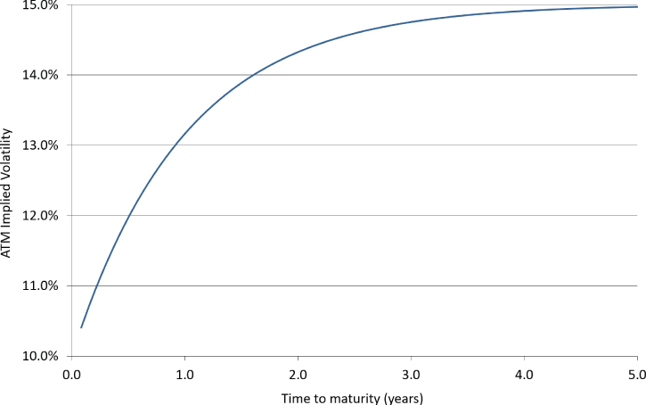
There are many possible ATM curve models. One of the simplest possible parameterizations introduced in Chapter 11 is:

where is the ATM implied volatility at time T (measured in years), and are the short- and long-term ATM volatilities respectively, and λ is the speed of reversion from to . This model can be implemented in an Excel sheet, with time displayed in monthly intervals (use 1/12 intervals within this stylized framework):

The output can be plotted in a chart:

The function can then be attached to the market expiry dates (and their T's) to calculate ATM implied volatility:

Task C: Adding Weights to an ATM Curve

In practice, traders keep their ATM curves aligned with the market by controlling the expected variance assigned to individual dates. This control is used to, for example, assign low variance to weekends/holiday days and high variance to major event days. One common way this can be achieved is by splitting variance into discrete daily chunks based on the weight assigned to each day.

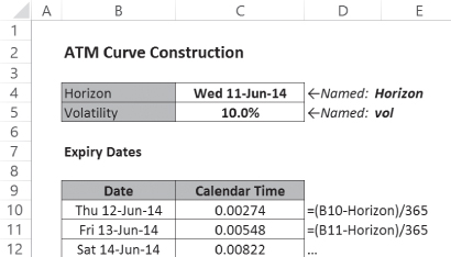
Within this model, a single flat volatility is used. By introducing a separate row for each date starting one day after the horizon (for at least a year), calendar time can therefore be calculated:

Day weights can now be added. These are defined in a table:

A VBA subroutine can be used to push the day weights onto the expiry dates. Note how the Weekday VBA function is cunningly used to generate the offset reference to the correct cell:

Sub populateDayWeights()
    Dim CountExpiryDates As Long
    CountExpiryDates = 1
    While Range("DateRef").Offset(CountExpiryDates, 0) <> ""
        Range("DateRef").Offset(CountExpiryDates, 2) =
          Range("DayWeightRef").Offset(Weekday(Range("DateRef").
          Offset(CountExpiryDates, 0)), 1)
        CountExpiryDates = CountExpiryDates + 1
    Wend
End Sub

The day weights up to a given tenor can then be summed and divided by 365 to calculate economic time. This calendar time versus economic time technique is used within real ATM curve models. Controlling economic time allows variance to be unevenly distributed over different days or, in more sophisticated models, over different parts of the day. For now, though, set weights of 1 on each day so calendar time and economic time are identical:

When weights are added, total variance to (calendar) time t changes from:

into

where dt = .

ATM volatility is then calculated from total variance using calendar time:

When plotted with constant day weights of 1, the ATM volatility is flat as expected:

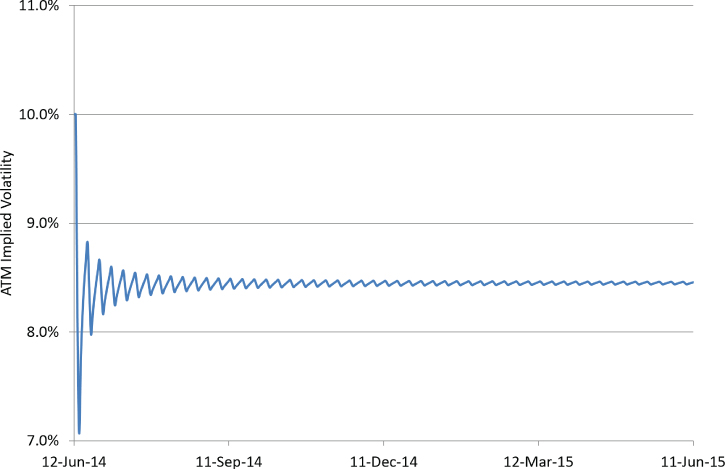
Now comes the magic: Set the weekend day weights to zero, repopulate the expiry date day weights using the populateDayWeights subroutine, and check the graph again:

The output now contains the ATM saw-toothing observed in the real FX derivatives market. Look at the data in the sheet:

In the model, economic time stops over the weekend because the FX market isn't open on Saturday or Sunday. In practice, trading desks usually assign a small but non-zero variance to the weekend because there is a small chance that unexpected news over the weekend will cause spot to move sharply first thing on Monday morning. The reduction in the economic-time-to-calendar-time ratio causes the ATM implied volatility for the Monday expiry to be lower than the Friday preceding it.

In this case, ATM volatility tends toward a value that is lower than the flat volatility input due to the ratio of economic time to calendar time being less than 1. In practice, this effect is adjusted for when there are target volatility levels that must be hit.

Finally, consider how the model is adjusted when there is an event. On Thursday, July 3, 2014, Non-Farm Payrolls (a big USD economic indicator, which normally occurs on the first Friday of the month) is released. Therefore, expected variance on that date is higher and the ATM volatility for that date is correspondingly higher. This is achieved within the model by moving the weight for that date higher:

The ATM volatility for the Non-Farm Payroll date itself moves higher plus the increased variance causes subsequent days to move higher, too. This is a real feature observed when building ATM curves: If expected variance for a given date increases, the ATM volatility for that date and subsequent dates rises:

Daily variance can now be calculated by taking the difference in variance between subsequent expiry dates, which in turn can be used to calculate daily ATM volatility. The daily ATM volatility is effectively the implied volatility for a strip of forward overnight ATM contracts. Traders use these forward overnight ATM volatilities to determine whether the ATM curve is overpriced or underpriced over events.

Vanilla FX derivative traders actively update weights within their ATM curve model to match market prices observed in the interbank broker market, plus future economic release dates are assigned higher weights when release schedules are known. Holiday days in a particular currency are known far in advance, too, and are assigned lower weights to reflect the reduced expected variance.

In practice, trading desks use frameworks similar to this but more granularity is usually included within the model. Exact times of events are often specified, enabling the correct pricing of different cuts within the same day. Trading desks also require a sophisticated core ATM curve, not just flat volatility. An approach similar to those developed in Task A or Task B in this practical will be usually be taken, with weights added on top in such a way that nonnegative forward variance is guaranteed.