Chapter 11
ATM Curve Construction
ATM curves can be constructed in two steps. First, a core ATM curve is established. Then additional parameters are introduced so the correct ATM implied volatility is generated for all possible expiry dates. Note that within this chapter, some calculations are approximate.
Variance
The key measure for building ATM curves is
where ![]() is the ATM implied volatility to time
is the ATM implied volatility to time ![]() (measured in years). For example, the variance of a 3mth ATM option with 12.0% implied volatility is
(measured in years). For example, the variance of a 3mth ATM option with 12.0% implied volatility is ![]() .
.
Variance can be thought of as a measure of cumulative spot movement. It has two powerful properties:
- Variance over any time period must be nonnegative.
- Variance is additive (i.e., variance over two days = variance on first day + variance on second day).
Variance can be used to calculate the forward ATM implied volatility (usually called forward implied volatility or just “forward vol” by traders) between two dates in the future. Given ATM implied volatility ![]() to time
to time ![]() , ATM implied volatility
, ATM implied volatility ![]() to time
to time ![]() , and
, and ![]() :
:
- Variance from horizon to

- Variance from horizon to

Therefore, variance between ![]() and
and ![]() and forward implied volatility between
and forward implied volatility between ![]() and
and  . For example, if the 6mth ATM implied volatility is 10.5% and the 1yr ATM implied volatility is 11.7%, then the forward implied volatility from 6mth to 1yr is
  .
.
Core ATM Curve Construction
There are two main approaches that can be used to generate core ATM curves:
- Input the ATM curve at the market tenors and interpolate to get ATM volatility for expiry dates between the market tenors.
- Use a model to generate the ATM curve and output the ATM volatility at the market tenors.
Recall from Part I that the standard market tenors up to two years are: O/N (overnight), 1wk, 2wk, 1mth, 2mth, 3mth, 6mth, 1yr, and 2yr.
Constructing a Core ATM Curve Using Interpolation
Core ATM curves can be constructed using interpolation between market tenors. Exhibit 11.1 shows ATM curve A—an upward-sloping ATM curve defined at market tenors.
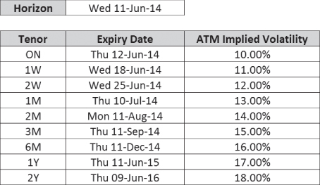
Exhibit 11.1 ATM curve A defined at market tenors
For expiry dates between market tenors, first consider linear volatility interpolation as shown in Exhibit 11.2. The linear interpolation methodology can be clearly seen between market tenors.

Exhibit 11.2 ATM curve A generated using linear volatility interpolation
To investigate this interpolation further, variance at each expiry date is calculated in Exhibit 11.3. The variance profile looks reasonable, rising over time as expected.

Exhibit 11.3 Variance profile for ATM curve A generated using linear volatility interpolation
Exhibit 11.4 shows a new ATM curve B defined at market tenors. ATM implied volatility is 20% at market tenors up to 1yr, and then the next data point is 15% implied volatility at the 2yr tenor.
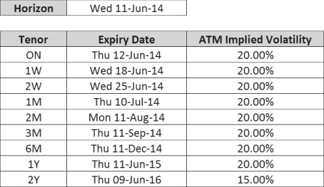
Exhibit 11.4 ATM curve B defined at market tenors
Interpolating ATM curve B using linear volatility and then calculating the variance at each expiry date gives the profile shown in Exhibit 11.5.

Exhibit 11.5 Variance profile for ATM curve B generated using linear volatility interpolation
Calculating daily variance (i.e., the change in variance for each expiry date) gives bad news in Exhibit 11.6.

Exhibit 11.6 Daily variance profile for ATM curve B generated using linear volatility interpolation
Up to 1yr, implied volatility is constant so variance rises linearly with maturity, but from 1yr to 2yr variance rises and then falls. This sets alarm bells ringing: Variance must be nonnegative. Therefore, linear volatility interpolation has failed to build a valid ATM curve from valid inputs (variance to 2yr is larger than variance to 1yr):
- Variance between horizon and 1yr = 20%2 × 1.0 = 0.04
- Variance between horizon and 18mth = 17.5%2 (interpolated) × 1.5 = 0.046
- Variance between horizon and 2yr = 15%2 × 2.0 = 0.045
This suggests a new interpolation methodology: linear variance. The variance profile resulting from a linear variance interpolation of ATM curve B is shown in Exhibit 11.7.

Exhibit 11.7 Variance profile for ATM curve B using linear variance interpolation
This variance profile has no negative daily variance and the ATM implied volatility curve shown in Exhibit 11.8 looks good, too.

Exhibit 11.8 ATM curve B generated using linear variance interpolation
Going back to ATM curve A, the profile shown in Exhibit 11.9 is generated using a linear variance methodology.

Exhibit 11.9 ATM curve A generated using linear variance interpolation
The ATM implied volatility between market tenors in Exhibit 11.9 looks odd. The linear variance methodology generates an ATM implied volatility profile that rises sharply initially and then flattens off between tenors for this upward-sloping ATM curve. Why is this happening? Consider the daily variance profile shown in Exhibit 11.10.
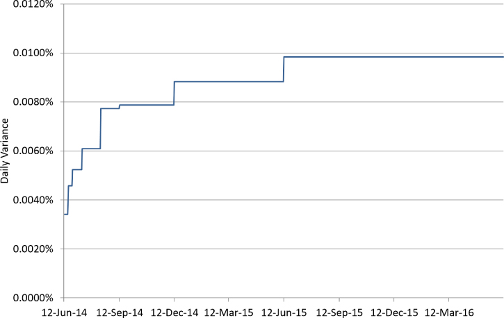
Exhibit 11.10 Daily variance profile for ATM curve A generated using linear variance interpolation
These daily variance patterns are not realistic. Intuitively it does not make sense that daily variance should jump immediately past each market tenor date. Excluding any special factors, why would daily variance one day prior to the 3mth tenor date be significantly different to daily variance one day after the 3mth tenor date? Ideally, the core daily variance function should be smooth.
Comparing these two interpolation methodologies:
- Linear volatility interpolation often produces intuitively correct ATM curves but does not ensure positive forward variance.
- Linear variance interpolation produces ATM curves that ensure positive forward variance (given valid inputs) but does not always create intuitively correct ATM curves.
In practice, trading desks use a combination of these approaches to produce intuitive curves with no negative forward variance. ATM curves are generally constructed in variance terms but more sophisticated schemes are used to control how daily variance evolves over time.
Constructing a Core ATM Curve Using a Model
Another possible method of constructing a core ATM curve is to use a model. Many different models are possible but fundamentally the functional form most often involves a short-term factor (could be volatility, variance, or daily variance), a long-term factor, and a speed of moving from short to long.
Here is one possible simple approach (that would never be used in practice because it could generate arbitragable ATM curves):
where ![]() and
and ![]() are short-term and long-term ATM volatilities respectively, λ is speed, and T is time to expiry measured in years.
are short-term and long-term ATM volatilities respectively, λ is speed, and T is time to expiry measured in years.
The ![]() function moves between 0 and 1 as shown in Exhibit 11.11.
function moves between 0 and 1 as shown in Exhibit 11.11.

Exhibit 11.11 Function used within a simple ATM curve model
Higher λ causes the function to move from 0 to 1 more quickly. This function can be fed with the T's from market tenor expiry dates to calculate ATM implied volatilities as per Exhibit 11.12.

Exhibit 11.12 ATM curve output at market tenors
The ATM curve is now an output from the model rather than being an input. This approach requires the model parameters to be calibrated to market ATM implied volatilities. This can be time consuming initially but traders soon learn how the model parameters change as the market ATM curve moves.
Within this approach, overrides at market tenors are also required to ensure the system ATM implied volatility hits market mid values. For example, the ATM curve model is set up and all tenors closely match the market except for 2mth ATM, which is 0.1% lower in the market than the model suggests. The trader therefore inputs a –0.1% override at the 2mth tenor. This is useful information because it suggests that the 2mth ATM is relatively cheaper than other tenors.
ATM Curve Construction: Short-Dates
Once the core ATM curve has been constructed, additional parameters or weights are introduced in order to give traders sufficient control over the curve. This control is required because different expiry dates (or even different times within expiry dates) have different expected spot volatility and this information must be incorporated into the ATM curve.
This additional control is mainly important at shorter expiry dates. The following examples demonstrate how the same variance framework can be applied at shorter time scales, as per the diagram in Exhibit 11.13.

Exhibit 11.13 Short-date variance examples framework
Example 1: 1wk (7-day) ATM implied volatility is 12.0%. A 1wk option always contains five weekdays and two weekend days where spot does not move because the market is closed (i.e., zero variance). Assume spot is equally volatile on each weekday (i.e., equal daily variance). What is the 8-day ATM implied volatility?

Example 2: 1wk (7-day) ATM implied volatility is 12.0%. Assume it is known that spot will be completely static during the 8th day (i.e., zero variance). What is the 8-day ATM implied volatility?

Due to the properties of variance, this effectively forms a lower bound on the 8-day ATM implied volatility: If the 7-day ATM volatility is 12.0%, the 8-day ATM volatility must be at least 11.25%.
Variance and option premium are closely linked. If forward drift and discounting are removed from the framework, the vanilla option premium for a specific strike must rise at longer maturities since variance must rise at longer maturities. Otherwise, the ATM curve is arbitrageable.
In practice, however, with forward drift reintroduced, the situation becomes more complicated. Consider vanilla options on two consecutive expiry dates with the same strike. If the following trading position can be achieved for zero premium, how can a guaranteed profit be generated from these trades?
- Short 7-day call option with strike K
- Long 8-day call option with strike K
If both options are left unhedged until expiry, profitability depends on how spot moves between the two expiry dates. An overall profit will be generated if spot is more in-the-money (ITM) at the second expiry than the first. However, an overall loss will be generated if spot is more ITM at the first expiry than the second. There is no guaranteed profit locked in.
A better strategy would be to sell the second option as the first option expires. This would offer a near-certain nonnegative P&L, but Exhibit 11.14 shows how an extreme forward drift prevents a guaranteed profit. The vanilla call option value at expiry (shown in leg 1) has a higher value than the second vanilla call option (now overnight expiry) due to the large negative forward drift.

Exhibit 11.14 Impact of forward drift on option prices
In practice it is hard to guarantee a profit on this trade, particularly once bid–offer spreads are taken into account. However, taking a step back, traders would love to transact this 7-day versus 8-day spread for zero premium. Traders often get carried away describing trades or prices as arbitrages when they really mean “fantastic trading opportunities.” As a result, the “arbitrage trading books” on bank derivatives trading desks can occasionally end the year with negative P&L.
Implied Volatility Patterns over the Week
The number of market-open and market-closed days to a specific expiry date has an important impact on the ATM implied volatility. Consider (one-day) overnight ATM volatility compared to the 1wk ATM volatility. Assume each market-open day is equally volatile (i.e., equal daily variance) and no variance over the weekend:

In words, the (one-day) overnight ATM implied volatility is higher than the 1wk ATM implied volatility because the 1wk expiry date contains two weekend days. This is a commonly observed feature of the FX derivatives market.
The market-open-to-total-days ratio also explains why ATM implied volatility tends to rise for future expiry dates over the working week. For a fixed horizon, a future Monday expiry will almost always have a lower implied volatility than the Friday following it because the Friday has a higher market-open-to-total-days ratio. This ATM saw-toothing, shown in Exhibit 11.15, is commonly observed within the FX derivatives market, although the effect dampens at longer maturities as the market-open-to-total-days ratio stabilizes.
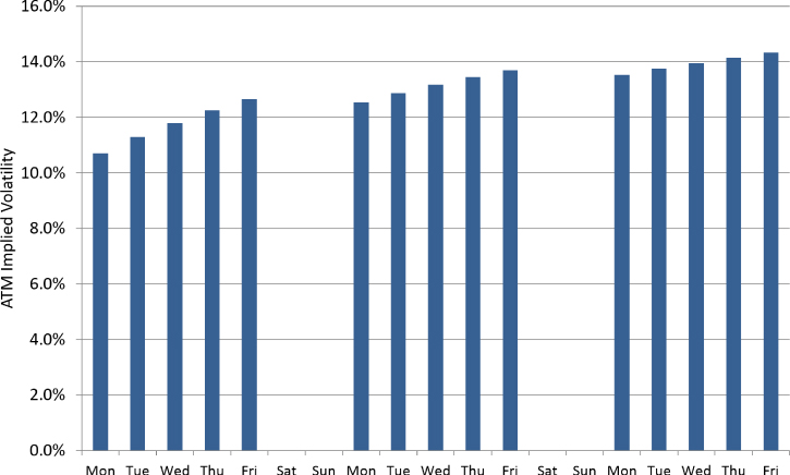
Exhibit 11.15 Monday to Friday ATM saw-toothing
FX Derivatives Market Pricing
Within the FX derivatives market, when using the Black-Scholes formula for pricing, time to expiry (T) is specified in discrete daily steps. This is a key feature of the FX derivatives market.
Consider a situation where the current time is 9 a.m. London time on Monday and overnight NY cut ATM implied volatility is 15.0%. The overnight expires tomorrow, so ![]() and:
and:
This variance can now be split into even smaller time intervals. NY cut is at 10 a.m. New York time, which is (usually) 3 p.m. London time, so this overnight option actually expires in 30 hours. Assuming spot is equally volatile between now and NY cut tomorrow:
After one hour passes, the remaining variance on the option is:
which implies a new overnight ATM volatility of:

Note that T is unchanged within this calculation due to being specified in discrete daily steps. At the start of each trading day, when the overnight option expiry moves forward one trading day, the ATM implied volatility jumps higher due to increased variance. Then over the course of the trading day, the ATM implied volatility gradually moves lower due to reducing variance. Variance (and hence premium) to a fixed expiry date reduces as time passes but because the market uses constant daily T values within the Black-Scholes formula for pricing, implied volatility reduces instead. This effect occurs at all tenors but the impact is only visible in short-dated options, particularly the overnight.
It is interesting to consider that if the market used a more accurate T for pricing, short-dated implied volatility would be more stable throughout the day. However, since spot volatility is not constant throughout the day, implied volatility would not be completely static. Therefore, introducing more accuracy into T adds to the complexity of the market for only minimal benefit.
In practice, short-dated implied volatility does tend to drift lower over the course of the day, but spot behavior is also important. If there is a large spot move or spot breaks out of its recent range, implied volatility generally moves higher due to an expectation of increased future spot volatility. Traders with short gamma positions come into the market to hedge their positions and the market implied volatility increases. Alternatively, if spot is static, implied volatility often falls more quickly than its “natural rate” as traders come into the market to reduce long gamma positions where they are struggling to trade their deltas.
If traders believe short-dated implied volatility is falling slower than it should over the course of the day, gamma can be “rented.” This involves, for example, buying the overnight ATM at the start of the trading day and then selling the same contract back at the end of the trading day. This technique is only applicable in liquid currency pairs where there is good two-way flow in short-dated vanilla options; otherwise the spread cross involved in the two transactions will kill any value in the trade.
Risk management of FX derivatives positions is also usually performed assuming discrete daily time steps. This is the reason that options expiring on the horizon date generate delta jumps through their strike level (as seen in Chapters 7 and 9). It is also the reason that trading positions show all options expiring on the horizon date at their own expiry times. If the trading position has options expiring at different cuts on the expiry date, this is inconsistent, but it keeps the trading risk stable. Traders adjust for this effect within their risk management.
Overnight (O/N) ATM on a Friday
On any weekday apart from Friday, the overnight option expires the following day. However, on Friday, the “overnight” option expires on a Monday; three days later rather than one. Therefore, in a market Black-Scholes pricing world, ![]() .
.
Vega ![]() is a function of
is a function of ![]() :
:
Therefore (ignoring discounting):
There is no volga ![]() on ATM options, so for a given tenor, roughly:
on ATM options, so for a given tenor, roughly:
Assuming there is no variance over the weekend and each weekday is equally volatile, the O/N ATM contract will have the same premium each day and therefore:

In practice this means that the market overnight ATM implied volatility quoted on a Friday cannot be directly compared with the overnight ATM implied volatility quoted on other days. To get the Friday overnight ATM into the same terms it must be multiplied by ![]() . Furthermore, the bid–offer spread shown on a three-day overnight should be tighter in volatility terms in order to show the same premium spread. Again, the level of ATM implied volatility is being impacted by the market-open-to-total-days ratio, or put another way, the ratio of economic time (time adjusted to consider market activity only) to calendar time (see Practical E).
. Furthermore, the bid–offer spread shown on a three-day overnight should be tighter in volatility terms in order to show the same premium spread. Again, the level of ATM implied volatility is being impacted by the market-open-to-total-days ratio, or put another way, the ratio of economic time (time adjusted to consider market activity only) to calendar time (see Practical E).
In practice, the market pricing of the overnight ATM contract on a Friday is closely related to the market's weekend decay position. The jump from Friday end-of-day to Monday morning covers three days. If this is not correctly adjusted for within risk management systems, theta from Friday to Monday will be artificially large. In a simplified world with no adjustment for this effect, a position that is long the same amount of gamma each day will, on average:
- Make money on Tuesday through to Friday as only (5 / 7) = 71% of the correct theta is paid per day.
- Lose all additional profit the following Monday as (5 / 7) × 3 = 213% of the correct theta is paid from Friday into Monday.
Amazingly, in a sophisticated financial market in the twenty-first century, this effect still produces trading opportunities as short-dated options can become too cheap on Friday as some banks oversell to reduce their weekend theta.
New York Cut versus Tokyo Cut Pricing
In G10 currency pairs the two most common expiry cuts are New York (NY) and Tokyo (TOK). The New York cut versus Tokyo cut ATM volatility differential can be analyzed using the same variance framework:
- TOK cut: 3 p.m. Tokyo time (often 6 a.m. GMT)
- NY cut: 10 a.m. New York time (often 3 p.m. GMT)
That is, NY cut options contain an extra nine hours of optionality.
Therefore, the Tokyo cut ATM implied volatility is always lower (“trades at a discount”) than the New York cut ATM implied volatility because both are priced using the same discrete daily ![]() but the Tokyo cut occurs first in the day and therefore has less variance and a lower premium.
but the Tokyo cut occurs first in the day and therefore has less variance and a lower premium.
Assuming spot is always equally volatile:

where ![]() is the time to expiry measured in years used within the market Black-Scholes pricing framework,
is the time to expiry measured in years used within the market Black-Scholes pricing framework, ![]() is the real time to expiry to the Tokyo cut and
is the real time to expiry to the Tokyo cut and ![]() is the real time to expiry to the New York cut.
is the real time to expiry to the New York cut.
Therefore, the New York cut versus Tokyo cut volatility differential increases over the course of a given trading day.
At 9 a.m. GMT:
- O/N TOK cut = 6 a.m. GMT the next day = 21 hours
- O/N NY cut = 3 p.m. GMT the next day = 30 hours

At 5 p.m. GMT:
- O/N TOK cut = 6 a.m. GMT the next day = 13 hours
- O/N NY cut = 3 p.m. GMT the next day = 22 hours

For maturities past three months, New York and Tokyo cuts will generally be priced at the same implied volatility (assuming no events, etc., on the expiry date). For example, at the three-month tenor, approximately:

Intraday Variance Patterns
The simplifying assumption that spot is equally volatile throughout the trading day is obviously not correct in practice. In liquid G10 currency pairs, realized variance follows a fairly well-established pattern shown in Exhibit 11.16 in which it:
- Starts low and builds up during Asia trading time
- Peaks around GMT 08:00 as Europe/London come in
- Dips during Europe/London lunch around GMT 11:00
- Picks up again in the afternoon with New York in and reaches day highs around GMT 14:00
- Decreases after GMT 15:00 (NY cut) to the end of the day in the New York afternoon

Exhibit 11.16 Stylized intraday hourly realized variance
The intraday variance patterns are different in emerging market currency pairs where trading is concentrated in one region or the spot market opening hours are restricted. Such variance patterns should be taken into account within the option pricing framework for maximum accuracy when pricing options expire at different cut times.
Events and Holidays
Events (economic data releases, election results, etc.) cause spot to move as the market adjusts to new information. Exhibit 11.17 shows the USD/JPY spot reaction to the Non-Farm Payroll data release (an important gauge of U.S. employment usually released on the first Friday on the month) from May 2013, in which spot jumps immediately after the economic data is made public.

Exhibit 11.17 USD/JPY spot over Non-Farm Payroll data release from May 2013
Event days are therefore assigned higher variance within the ATM curve, specifically in the period immediately after the data is released. This in turn increases the ATM implied volatility for options expiring on that expiry date (if the cut occurs after the event has been released) and also expiry dates following it. The exact date and time of events is known beforehand and therefore the market ATM curve incorporates this information.
On days containing important data releases, realized spot variance is usually similar or slightly lower than the spot variance on a “normal day” until the data release. Over the data release, realized spot variance increases sharply and then reverts back to the normal day as shown in Exhibit 11.18. On this expiry date, the NY cut contains the additional expected spot variance from the event but the TOK cut does not. This leads to a far larger NY cut versus TOK cut ATM implied volatility differential than usual.

Exhibit 11.18 Stylized intraday hourly realized variance on Non-Farm Payroll day
The presence of an event also causes short-dated implied volatility to decay differently over the course of the day. Prior to the event, short-dated ATM implied volatility will move lower only slightly but after the event has occurred ATM implied volatility can drop sharply as expected future spot variance reduces.
Events usually occur in a particular currency. For example, European employment data primarily impacts spot in currency pairs that include EUR. However, for the most important events, crosses can also exhibit increased volatility if the majors move in an asynchronous manner. For example; Non-Farm Payrolls impacts USD, but if EUR/USD and AUD/USD are both more volatile but they do not move in a perfectly synchronized manner, EUR/AUD realized volatility also increases.
Public holidays also impact realized volatility and variance. There is often significantly less spot activity in pairs containing the holiday currency simply because there are fewer market participants operating that day. In addition, U.K. and U.S. public holidays are important enough to reduce spot activity across all currency pairs. Therefore, public holiday days in a particular currency have lower variance within the ATM curve.
Weekday Variance Patterns
The FX spot market often exhibits increased realized variance later in the working week, as shown in Exhibit 11.19. This effect occurs partially because there tend to be more data releases later in the week. However, even with the effect of events removed, Mondays are often less volatile than other weekdays.
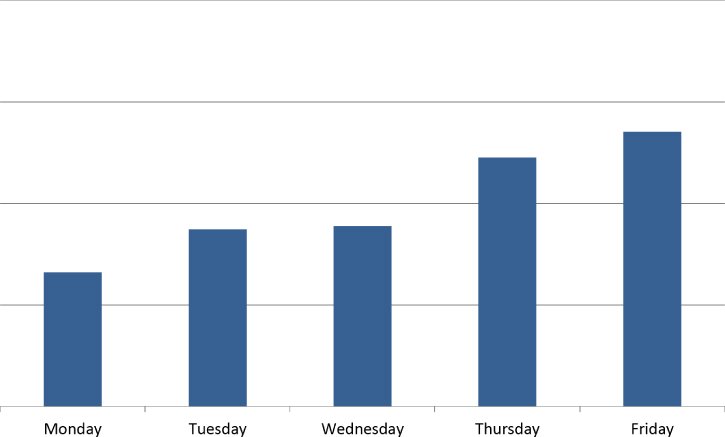
Exhibit 11.19 Average daily spot variance for G10 pairs in 2012
Like the NY cut versus TOK cut implied volatility differential, the day of the week of a particular expiry date matters more at shorter tenors than at longer tenors. The market often has a preference to buy the next few Friday expiries and sell the next few Monday expiries but the weekday of, for example, the 6mth ATM contract is not a major concern.
Pricing Same-Day Options
Pricing options that expire later today is impossible within the standard market Black-Scholes pricing framework. The number of days is zero; hence T is zero and therefore same-day options cannot be quoted in volatility terms. Recall from Chapter 5 that in the Black-Scholes option pricing formula:  would break because the denominator is zero.
So-called same-day options must therefore be quoted in premium terms. One way to calculate the premium of a same-day option is to start with an overnight option and use the variance framework to adjust the implied volatility.
Example: At 9 a.m. GMT a client requests a price in a same-day NY cut option. This is shown in Exhibit 11.20.

Exhibit 11.20 Pricing a same-day vanilla option
The O/N NY ATM implied volatility is 12%. Therefore:
Assuming each hour has equal variance:
Therefore, the equivalent one day ATM volatility is:

This implied volatility can then be used to price an overnight option which gives the same-day option premium. Note that interest rates should be set to zero within the same-day pricing since forward drift and discounting will have no impact.
In general, same-day options are nonstandard and a wider bid–offer spread should be charged. Plus it is vital to take expected intraday variance profiles and events into account. Be suspicious: Why wouldn't the counterparty be happy to wait until the standard option expiry time?
