The focus of this book is on the valuation of properties and development projects in the face of uncertainty. We concentrate particularly on management and design flexibility, which is the ability to respond to circumstances in order to reduce downside risks and take advantage of upside opportunities.

To this end, everything in this book builds on and uses the basic discounted cash flow (DCF) model. So, to ensure we’re all on the same page, and using the same terminology and basic understanding about this tool, this first chapter introduces and reviews the DCF model, and thereby sets the stage for all that follows.

First, we discuss why it makes sense for us to focus on the DCF model. What makes the DCF model so appropriate for our purpose? (See Section 1.1.)

Second, we describe the essential elements of the DCF model. We define both the terminology and structure of the model that we use throughout the book. We do this to establish a common vocabulary and to avoid confusion that might arise from different professional practices. This quick review also introduces DCF modeling for those who might not be familiar with the procedure (see Sections 1.2–1.4).

Third, we illustrate the two basic ways to use the DCF model to value projects. We can use it to value projects prospectively—in advance of making investments, as an aid to decision‐making. We can also use it retrospectively—to assess the actual past performance of a real estate asset and investment, to help diagnose the causes of success and failure (see Sections 1.5 and 1.6).

1.1 Why the Focus on the Discounted Cash Flow Model?

Three factors make the DCF model the most appropriate basis for valuation of real estate properties and developments in the face of uncertainty:

• DCF is based on fundamental financial economic theory, explicitly recognizing and valuing, based on opportunity cost, the three seminal considerations in investment: cash flow, time, and risk.
• The DCF model is already the analytic workhorse for valuation of real estate investments. Many of you are probably already familiar with it.
• Implemented in modern computer spreadsheet software, the DCF model is very efficient and widely applicable. The relevant calculations usually take seconds or less. And the model can realistically represent a wide range of complex situations useful for valuing flexibility under uncertainty.

Allow us to elaborate briefly on these three points.

The focus of DCF on cash contrasts with a focus on accounting metrics such as net income. Of course, such accounting metrics are very important, and DCF models often include and use accounting metrics. Nevertheless, cash is what you can actually use—in investments, in business, in life. The accounting metrics are indirect representatives, reflections, or predictors of the existing or future cash flow that ultimately matters.

The “D” part of “DCF” is how we account for time and risk in the valuation. Future money is worth less than present money for two reasons:

1. You could be using the money in the meantime (maybe to spend on consumption, maybe to earn returns in investment); and
2. The future money might not materialize in full or at all, since the future is uncertain (no one has a crystal ball).

The discount rate by which the DCF procedure reduces future expected cash flow to present value (PV) accounts for both of these considerations. It does this accounting based on the fundamental economic principle of opportunity cost, using a discount rate that reflects what the investor could expect to earn by investing in a similar investment of similar risk. In short, the DCF model is solid, elegant, and intuitive.

The DCF model is not just sound from an economic theory perspective—its use too is widespread. DCF models operate using computer spreadsheets, which are a common way to organize data for valuation analysis. Spreadsheets are everywhere in financial analysis. Business analysts and decision‐makers worldwide use common spreadsheet programs such as Microsoft Excel^®. Such spreadsheet software is, in effect, a common language in the business and financial world. This can greatly facilitate communication, transparency, understanding, and use.

Finally, DCF models based on computer spreadsheets have tremendous range and flexibility in what they can do for us analytically, especially in our quest to bring uncertainty and flexibility explicitly into valuation. Spreadsheets take in numerical data and calculate outputs, allowing us to easily change one or more entries and recalculate to see the results instantaneously. Spreadsheets have two special capabilities that enable us to represent uncertainty and flexibility. These capabilities are easy to implement and use, and are essential to the approach we present in this book.

• First, we can easily use spreadsheets to calculate thousands of variations of the same problem automatically, in seconds. This feature allows us to deal with the range of possible economic and other variations that could affect the performance of an investment and hence the valuation of the real estate. This frees us from the need to confine our analysis to just a few estimates of the possible future. It enables us to look at probabilistic distributions of possibilities in detail, such as the effects of business cycles and market movements—a step that is necessary for the proper valuation of flexibility. This capability is available through the random number generation capability and the “data table” function in Microsoft Excel^®.
• Second, we can set up the spreadsheet to represent the actions of a decision‐maker choosing to take appropriate actions under the conditions we specify. In effect, we can create an analog model of the investment and decision‐making process. Thus, we can program potential decisions to take advantage of the flexibility to sell a property under favorable circumstances, or to delay development in a down economic cycle, for example. This capability enables us to represent and quantify the advantages of certain options and certain types of decision flexibility. This approach also enables us to value several options simultaneously, a capability largely beyond the ability of many of the formal academic models of option valuation. In essence, we employ “IF statements” in Microsoft Excel^® formulas.

1.2 Structure of a Discounted Cash Flow Spreadsheet

Let’s now review the widely accepted and somewhat standardized structure and procedure for the DCF analysis we use for valuation, arguably a canonical framework in real estate. As we have said, this structure is tailor‐made for spreadsheets (and vice versa). It is usual to call this setup and framework a “pro forma analysis,” or, simply, a DCF “pro forma.”

Table 1.1 presents a simple numerical example of such a DCF valuation for a stylized commercial rental property. As Table 1.1 illustrates, the DCF pro forma is a table (or matrix) showing the state of an investment over time in two dimensions (rows and columns). The overall structure is that:

• The columns specify different periods, for example, years. For generality, a usual practice is to number the columns starting with “0,” which refers to the present—that is, the time when the analysis and evaluation are applicable. “Column 1” is the first year (or period) in the future, “Column 2” the second, and so on.
• The rows represent revenue and expenditure items relevant for analysis and valuation. We speak of these as the “cash flow over time” of the line item represented in the row. The normal convention is to assume that cash flows occur “in arrears”—that is, as of the end of the indicated period. Some rows are sometimes used to display the underlying physical source amounts, such as the quantity of units sold or the square meters of space occupied.

1.3 The Cash Flow Projection

In this and the next sections, we review the essential mechanics of the DCF valuation procedure. We first focus on the future stream of cash flow we expect from the property—that is, the estimates of its future revenues and expenditures, period by period. It’s important to note that we specify these estimates by period. It isn’t enough to estimate the overall revenues and expenses; one must assess how they evolve over time. This is because the discounting process noted previously (and as elaborated in the following section) will give different present values to future cash flows, depending on how far in the future they occur.

We base cash flow projections on a variety of sources. These include:

• Knowledge of fixed contractual obligations (such as mortgage payments and lease terms);
• Informed best estimates of specific income and expenses; and
• Assumptions about the relevant real estate market and overall economic conditions, such as future prices.

Table 1.1 presents a simple numerical example of a commercial rental property, in which the cash flows are all speculative estimates. You might think of the property as an apartment property.

Later in this book, we focus primarily on development projects—that is, investments that require considerable construction up front as well as possibly in later stages. Development projects can have major net negative cash flows for extended periods or at different times during the project’s life. But, to begin, we focus on a simpler and more fundamental type of capital asset, as represented by the fully operational rental property depicted in Table 1.1. (A fully operational property occupied to a normal level is also referred to as a “stabilized” property.)

The property owner takes in rental revenue and pays out cash to cover operating and capital expenses. The difference between the money in and the money out is the “net cash flow.” This can be either positive or negative in any given period. Positive cash flow means that the property owner receives money, net, from the asset. Negative cash flow means that expenditures exceed revenues, and that the property owner must somehow provide cash to the property.

While we have not labeled the cash flows in any particular currency, we refer to them in “dollars” for illustrative purposes. Note also that Table 1.1 uses real estate terms typical for the United States.

Table 1.1 projects all the estimated cash flow components in our property to grow at a steady rate. This practice does occur in the real world as a simplification, but here this simplification is for ease of illustration, to allow us to make some essential points more clearly. For the property in our example, we use a projected growth rate of income and expenses of 2% each year, as indicated at the top of the spreadsheet. While this might be a typical rate of growth for rental property in a mature economy, it is just an example of growth projection.

It is usual to structure the rows so that annual revenues are generally at the top of each column, followed by costs, leading to net cash flow for the year at the bottom. Table 1.1 is reasonably standard in this respect. To see how this works, consider the entries in the column for Year 3. Taking each row in turn, we have:

• Potential gross income (PGI): This refers to the revenue that the property would generate if it were fully occupied. (This is also sometimes referred to as Gross Revenue, or Rent Roll.) We project this as $104.04 in Year 3, which is the $100 of Year 1 grown by 2% over 2 years.
• Vacancy allowance: This implies that some fraction (which we assume to be 5%, or $5.20) of the potential revenue will not be generated, owing to vacancy in the property during the year.
• Effective gross income (EGI): $98.84 equals PGI minus vacancy allowance.
• Operating expenses: This refers to the estimated regularly recurring costs for operating the property, such as utilities, insurance, property taxes, maintenance, and management costs.
• Net operating income (NOI): $62.42 equals EGI minus operating expenses.
• Capital improvement expenditures (“Capex”): This refers to the longer‐term, less regularly recurring expenditures incurred to improve the property and keep it running—for example, a new roof, new heating or air conditioning system, repaving the parking lot or re‐landscaping the grounds, refurbishing and refitting apartments with new appliances, etc.
• Net cash flow: $52.02 equals NOI minus Capex; this is the overall difference between the money in and the money out, at the property level. (In this book, we focus on the asset level, not considering specifically investor‐level cash flows such as debt payments or income taxes—although, of course, the DCF model may also be applied at that level.) Net cash flow is our “bottom‐line” projection for operations in Year 3. As noted, the net cash flow can be either positive or negative in any given year.

A complete DCF valuation, in addition to its ongoing annual cash flows, has to account properly for the projected value of the asset at the time it might be sold. We do this by projecting what real estate analysts call the “reversion” cash flow. This amount corresponds to what in other fields of capital budgeting might be termed “terminal value” or “salvage value.” In real estate, this is the expected resale price for the property.

In practice, real estate analysts usually consider that the resale of the property will occur at some finite horizon, often using the nice round number of 10 years. (Many leases and mortgages have terms equal to or less than 10 years, and many owners in fact resell investment properties after about that length of holding.) We can use other horizons, but Table 1.1 conventionally calculates the reversion cash flow with the standard 10‐year horizon.

The reversion is logically the capitalized value of the future stream of net cash flow that the property will provide beyond the resale horizon date (the present value for the next buyer). The common way to estimate this is to divide the projected net cash flow for the year beyond the resale horizon (in our case, Year 11) by a projected cash yield rate for that time. Thus:

(1.1)

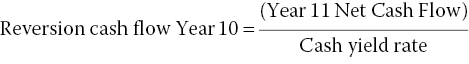
This “ratio valuation” formula is a practical, acceptable procedure for reversion valuation. It skips the full, multi‐year DCF valuation, which might require difficult or excessively speculative projections beyond the 10‐year horizon.

Our example assumes a “going‐out” (or “terminal”) yield rate of 5% for a valuation as of the end of Year 10 (which is therefore applied to the projected cash flow of Year 11). Thus, the estimated Year 10 reversion cash flow equals the Year 11 projected net cash flow of $60.95 divided by 0.05, which is (rounding out) $1218.99, shown as reversion in the Year 10 column.

The overall bottom line for our DCF valuation model in Table 1.1 consists of the operating net cash flow amounts during the first 9 years plus, for the terminal tenth year, the sum of its operating cash flow and the projected reversion. Thus, the Year 10 net cash flow projection is $1278.75 (operating net cash flow of $59.75 plus the projected reversion of $1218.99).

We now have all the cash flow data needed to perform the DCF valuation analysis. To value the asset, in addition to cash flow, we need another crucial parameter: the discount rate. Let’s think about what this should be.

1.4 Discount Rate

The role of the discount rate—that is, how the DCF valuation accounts for time and risk—was noted in Section 1.1. The discount rate has its name because it discounts—that is, reduces the value of—future amounts in terms of the present value (PV). The formula for this reduction is:

(1.2)

These reductions can be huge. Figure 1.1 illustrates the phenomenon, showing how several discount rates reduce the value of $100 received in future years.

What should the discount rate be in our DCF valuation? This is a most important issue, since the rate strongly affects the perceived economic value of the project. As noted in Section 1.1, for market valuation purposes, the discount rate should equal the opportunity cost of capital (OCC). We discuss this important concept in some depth in Chapter 2. For the moment, we assume in Table 1.1 that the appropriate discount rate is 7% per year.

1.5 Market Value and Forward‐Looking (Ex‐Ante) Analysis

We can now value the asset. In terms of mechanics, once we have set up the spreadsheet, filled in our estimates of cash flows, and selected the discount rate, all we have to do is place the proper formula in the desired cell and initiate calculation. In our example, the result is the $1000 value that appears in the bottom left‐hand corner. This is the present value (PV) of the property. It is the value of all the net future cash flows placed on the common basis of the present, controlling for time and risk.

In detail, the calculation works as follows. (These steps are not visible on the pro forma.) The computer spreadsheet reduces the net cash flow in each year to its present value and sums up the result across all the years; this equals the value of the asset. The reduction for any year depends on a compounding of the discount rate by the number of years between it and the present, as Equation 1.2 indicates. Thus, Year 1 net cash flow of 50.00 reduces to the PV:

Year 2 net cash flow of 51.00 reduces to the PV:

And so on. Finally, the PV of the Year 10 net cash flow is:

The sum of all these present values of the future cash flow expectations is:

This DCF valuation is forward‐looking; that is, its data come from projections of future years’ cash flows (including the resale). It is a typical pro forma application of the model that is appropriate for evaluating a property asset at the present time (Time 0). This is because the present value of the asset depends on the net cash flow that we anticipate it to produce in the future. We refer to this as an “ex‐ante” analysis. This way of using DCF valuation is typical for estimating the “market value” of a property asset, presuming the cash flows are unbiased estimates and the discount rate is a realistic estimate of the market OCC. The market value is an estimate of what the property would sell for. Ex‐ante DCF analysis is also useful to estimate “investment value,” which is a private valuation for a particular investor. Investment value may differ from market value if the investor differs from the typical marginal buyer in the market, or if the investor knows something that the market does not know.

1.6 Backward‐Looking (Ex‐Post) Analysis

We can also apply the DCF model to a past investment. In this case, our cash flows are historical—they have already happened—so we use actual amounts rather than estimated future amounts. We might do this as part of a retrospective, “post mortem” analysis of an investment. We refer to this as an “ex‐post” analysis.

The spreadsheet for the ex‐post analysis of a project has the same structure as Table 1.1. However, the year headings at the tops of the columns would refer to specific past years, and the cash flow amounts in the table would equal the actual recorded historical cash flows in those years.

The focus of the ex‐post analysis differs from that of the ex‐ante analysis. The ex‐ante analysis often aims to estimate the value of an investment, for example, so that we can have an idea of how much to pay for it, given the current opportunity cost of capital. In the ex‐post analysis, we know what we paid for the investment, and can apply the DCF to learn what rate of return we actually achieved. This can be helpful in conducting diagnostics, to learn the causes of investment successes and failures.

In later chapters, we introduce another way to use the DCF model in an ex‐post manner. We will create scenarios of future cash flow streams that could conceivably happen; in effect, we will calculate possible “future histories.” We can use the present values of these scenarios as a metric of interest in our simulation modeling. In effect, we will be conducting ex‐post DCF analyses of the possible future scenarios. The distribution of possible future ex‐post results then effectively presents us with an ex‐ante probability distribution.

1.7 Conclusion

This chapter introduced (or briefly reviewed for you) the discounted cash flow valuation model, perhaps the most basic construct in property valuation, and in the tools we present in this book. We discussed the basic rationale, terminology, and mechanics of the model, and pointed out how it may be used in either a forward‐looking or backward‐looking manner. The next chapter deepens this discussion by going further into the economics of the model.