This chapter explains the concepts needed for a good economic valuation of a real estate property or development, and distinguishes between the various terms used in this process. You may think of this chapter as the conceptual counterpart to the discussion of the mechanics of discounted cash flow (DCF) in the preceding chapter. It is our opportunity to make sure that we are all on the same page regarding the basic concepts and meanings associated with the valuation of real estate and use of the DCF model.

2.1 Choice of Discount Rate

Mechanically, the discount rate we use in the DCF valuation model simply converts future cash flow amounts to present values (PVs). But the economic meaning of this mechanical process can differ depending on what the future cash flows represent and on what type of value is used for the discount rate.

If, as is usually the case, we are interested in estimating the “market value” (see Box 2.1) of the asset, then the future cash flows should represent unbiased expectations, and the discount rate should equal the “opportunity cost of capital” (OCC) faced by investors dealing in the market where the asset is traded. Anyone who invests in our project or property asset is foregoing investing in other similar investments, and therefore is foregoing the opportunity to earn the returns that such alternative investments could provide. This is the sense in which the potential buyer of our property faces an “opportunity cost.” Therefore, to be competitively attractive, the expected return on our project should equal this opportunity cost, namely, the expected return on other assets of similar investment risk.

In practice, we can never know the exact OCC for any property precisely and definitively. It is not something you can just look up on the Internet! We can estimate the OCC based on surveys, experience, guidance from expert reports, relevant historical and market data, and our own understanding of the market and its investment opportunities, as well as our understanding of the risk of the project. Importantly, we are looking to represent what the market requires as an expected return, and not necessarily what we ourselves personally might think it should be.

In this regard, assets (investments) that seem more “risky” (in some sense) command higher expected returns; that is, they have higher OCC, relatively speaking. This is a widely documented market phenomenon. It is worth reiterating that this means that the OCC for a project that we are analyzing should equal the return on investment of properties with similar risk.

While this is the classical framework and is certainly true and good practice, we would be naïve not to raise another consideration. In many asset markets, the OCC depends on the competition for investment projects. This is related to the classical risk/return concept. But it does add an important additional perspective. The fact is that the OCC can reflect capital flows, which reflect the overall demand for real estate investment. Are there many good opportunities available? Is there a flood of investors with a lot of money looking to make investments? Is the central bank keeping interest rates very low? An abundance of good investment opportunities with a scarcity of investors will result in relatively low asset prices (as the projects compete with one another for scarce investment capital), and this will increase OCCs generally (picture a rapidly growing, emerging market country). In contrast, a flood of money will drive up asset prices and reduce OCCs as the ability of the assets to generate future operating profits remains largely unaffected by the capital inflow (picture the US commercial property market in 2007 or 2017). This money flow consideration can explain a lot of the variation over time, and between countries, in the typical magnitude of OCC rates applicable to real estate project valuation.

2.2 Differences between Discount Rate, Opportunity Cost of Capital, and Internal Rate of Return

Having introduced the construct of the discount rate and the concept of the OCC, we need to define and distinguish a third related metric, the internal rate of return (IRR). Students and practitioners often confuse these three terms (discount rate, OCC, IRR). Indeed, they are related. It can therefore be helpful for sharp, analytical thinking to try to grasp the subtle distinctions between these three constructs.

The discount rate is just a mechanical device. It is the rate we use to reduce future values to present values. There is not necessarily any normative implication in the term “discount rate.” In other words, someone might posit or use some rate as the discount rate, whether or not that rate has any particular economic meaning. For example, a corporation might dictate a “hurdle rate” as a management tool (but defined somewhat arbitrarily from an economic perspective), to be used as the discount rate in benefit–cost analyses for capital budgeting.

In contrast, the OCC is a normative economic construct. It is the rate that, when we employ it as the discount rate, gives a present value equal to the estimated market value of the asset (assuming the future cash flows are correctly estimated). This is because, as discussed in the previous section, the OCC represents the return that the investor could expect to get from investing in a typical asset with similar risk and return as the subject asset, in the asset marketplace, simply by paying market value for the asset.

The third construct, the IRR, is like the discount rate, in that it is not a normative construct but merely a mechanical or mathematical device. It is simply a way of measuring investment returns when the investment involves multiple cash flows occurring in several future periods. By definition, the IRR is the rate that discounts a stream of cash flows to an NPV of zero. Equivalently, if the investor has an upfront negative cash flow (having paid for the asset at the beginning of the investment), then the IRR is the discount rate that causes the resulting present value of the subsequent complete project cash flow stream to equal the magnitude of that initial investment amount or asset price. Thus, IRR is the discount rate such that:

(2.1)

To illustrate the concept of the IRR, let’s refer to the DCF analysis in Chapter 1. In that case:

• We made the discount rate 7%;
• We then derived a present value (PV) for the project, $1000;
• If 7% is the OCC, then $1000 is the estimated market value (MV);
• An investor who bought the project for $1000 would obtain a net present value (NPV) of: ;
• So, the investor’s implied expected return equals 7%, expressed as the IRR of the investment at the given price of $1000.

The preceding scenario is an example of an ex‐ante IRR, an expected future return computed going into the investment (also referred to as a “going‐in IRR”). On the other hand, computing the realized IRR in an ex‐post DCF analysis is a way to measure how well the investment performed. For example, one can compare the achieved IRRs across different investments. (However, in making any such comparisons, we shouldn’t forget our previous point that more risky investments should provide higher returns, on average and over the long run.)

Thus, to summarize: if you discount at the OCC, the present value you obtain will be the estimated market value (assuming unbiased projected cash flows). If you then pay a price equal to that market value, your going‐in IRR in the investment will be the OCC, the fair return given the amount of risk.

2.3 Net Present Value

The net present value (NPV) is the value of what you’re getting minus the value of what you give up to get it, evaluating the benefits and costs in “apples‐to‐apples” money terms—that is, controlling for time and risk (reflecting opportunity costs). Formally, the NPV of a project is the excess of its present value (PV) over its investment cost, which is often simply the price paid (P) for the asset. Thus:

(2.2)

To illustrate the concept, we build upon the DCF example from the preceding chapter. We assume that the cash flow projections remain as in Table 1.1 (including the reversion). However, we now suppose that the correct OCC is 6%, not the 7% discount rate employed in Table 1.1. In other words, we suppose that the investment marketplace has “decided” that it only needs a 6% return for assets like our subject property (perhaps interest rates have fallen, or the property is now viewed by the market as being less risky). In that case, the market value of the property, the sum of the present values of all the future cash flows discounted at 6%, would be $1080. At the lower discount rate, future expected cash flows are more valuable in the present, and the PV is higher than the $1000 calculated for a discount rate of 7%. But if we could still buy the property for $1000 (somehow, even though its market value is $1080, perhaps owing to the seller being misinformed or distressed), then our NPV would be: .

The existence of a positive, non‐zero NPV based on market value indicates that the investment is a bargain for the investor. It provides above market‐expected returns. Another way of arriving at the same conclusion is to observe that the ex‐ante IRR of the project at the $1000 price is still 7% (that is, the going‐in expected total return on the investment), and this is greater than the OCC of the investment, which is 6%. In general, in the market, you could not expect to buy other assets of similar risk at prices that would present you with more than a 6% going‐in IRR.

In most well‐functioning asset markets, it is hard to find such “bargains.” The definition of “market value” is that the property owner can expect to sell at that price. If the market value were $1080, why would the owner sell for $1000? In fact, paying a price equal to the (estimate of) market value provides . From such a market value perspective, this is not a “bad deal” for the investor (for the one buying or the one selling). From the market value perspective, the buyer receives , while the seller receives , where P is the price, and MV is the market value. Buying the asset for a price equal to its market value provides the investor with an expected return equal to the OCC, a “fair return” (ex‐ante). Nevertheless, in real estate and some other circumstances, non‐zero NPV deals can occur, even when evaluated from a market value perspective. In part, this is because it is usually difficult to know exactly and precisely what the OCC is or what the market value is of any given asset.

Non‐zero NPV opportunities are probably more common when the investment involves construction of new assets, as such entrepreneurial actions often create value. Of course, such development projects can be quite risky.

Perhaps a more common way for non‐zero NPV to occur, and, in particular, for positive NPV to occur, is to measure the NPV not from the perspective of market value but from that of some relevant type of “private value” (as defined in Box 2.1). Viewed from the private value perspectives of both parties, it is possible for NPV > 0 for both sides of the transaction, since the two parties’ private values may differ (and they transact at a price above the seller’s valuation and below the buyer’s). If we let “IV(B)” be the buyer’s “investment value” (as defined Box 2.1) and “IV(S)” be the seller’s investment value, then a typical real estate transaction might look like this:

(2.3)

And, the NPV from the buyer’s investment value perspective is: NPV(B) = IV(B) − P = IV(B) − MV > 0; while, from the seller’s perspective, it is: NPV(S) = P − IV(S) = MV − IV(S) > 0.

2.4 Relationship between Discount Rate, Growth Rate, and Income Yield

Now, let us stand back from the details of the DCF spreadsheet to consider some general relationships that will help you understand the terminology and basic economics of the DCF valuation model. In particular, let’s focus on the three rates involved in the basic DCF analysis: the discount rate, r; the growth rate, g; and the going‐in net cash yield rate, y. In a stylized model that simplifies but retains the important essence, the discount rate is the sum of the growth rate and the going‐in cash yield. In equation form, we have:

(2.4)

In the case of the illustrative DCF that we discussed in Chapter 1 (with the 7% discount rate), we have: , , and .

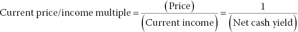
At this point, a few words about the net cash yield are in order. It is the ratio of current income to price:

(2.5)

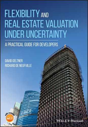
In our example from Table 2.1 (from Chapter 1), the net cash yield is the “going‐in” yield at the start of the project:

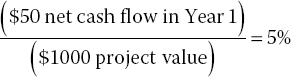
It is also the “going‐out” yield at end of the projected investment:

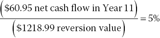
That both yields are 5% reflects (and helps to cause) the fact that our asset value is a constant multiple of its current income.

Note that the cash yield rate is simply the inverse of the asset’s current price/income multiple (which is another way of quoting asset prices):

(2.6)

Box 2.2 contains more detail on the various conceptions of yield in the United States and United Kingdom. It is a useful reference, which you can easily skip if you want.

2.5 Relationship between Discount Rate and Risk

Continuing with our elaboration of the basic DCF constructs, let’s expand on our previous point that expected returns are related to risk. We can express the discount rate as the sum of two factors, a risk‐free interest rate (rf) and a risk premium (RP):

(2.7)

The risk‐free interest rate is what investors can get by investing without any risk, such as perhaps in government bonds. If r is the OCC for the investment, then the RP in Equation 2.7 represents what the asset market “offers” to investors as the amount of extra expected return (ex‐ante) that compensates investors for taking on the risk associated with the given investment. (Of course, the market’s ex‐ante RP may not materialize ex‐post; that is what we mean when we say the asset is a “risky” investment!)

Putting Equations 2.4 and 2.7 together, we see that the investment cash yield is:

(2.8)

In other words, the yield is the sum of the rf prevailing in the economy, plus the RP reflecting the amount of risk in the subject asset as perceived (and priced) by the investment marketplace, minus the growth expected in the asset cash flows and future values.

These relationships make sense:

• The higher the interest rates are, the greater in general is the opportunity cost of investing in any one asset (thereby foregoing investing in any other asset); and hence, the lower the price/income multiple will be (higher yield).
• The riskier the asset, the more investors will demand a higher expected return; and hence, again, the lower the price/income multiple must be (other things remaining equal).
• Finally, the greater the expected growth in the asset’s future cash flow and value, the more the investor will pay per dollar of current net income; that is, the higher the price/income multiple will be, given that future income is expected to grow more.

These relationships are fundamental and important in the real world. While we present them as coming from Equations 2.4 and 2.7, we should point out that Equation 2.4 holds exactly only if the asset’s cash flows grow in perpetuity at a constant rate (the rate g), and the asset value will always be a constant multiple of its current cash flow level. Nevertheless, the above general points still hold in the real world even if Equation 2.4 is not true exactly.

2.6 Conclusion

This chapter elaborated some of the basic constructs and mechanics of the DCF model introduced in Chapter 1 to reveal some important economic considerations. We hope you can see that the DCF valuation model is essentially intuitive, as well as rigorously based in solid economic theory, at least, as far as it goes. The model provides a good basis and tool for us to use in the remainder of this book.