22
Project Phasing Flexibility: We Show How to Model and Evaluate the Delay Flexibility Inherent in Project Phasing
In Chapter 20, we saw that modular production timing flexibility can add substantial value to a multi‐asset development project. But, for many real estate development projects, the modular type of production flexibility is not realistic. However, it is widely possible to divide a large, multi‐building project into two or more distinct, pre‐planned “phases.” As described in Chapter 15, phasing flexibility involves a plan to produce parts or sections of the overall project separately, with each phase being able to function independently if necessary. Indeed, the phasing of large projects is quite common. Such phasing generally brings with it considerable timing flexibility—in particular, to delay the start of subsequent phases beyond the base plan schedule represented in the original pro forma. We now explore this subject by considering a modified version of our example Garden City project.
22.1 Modeling the Sequential Phase Delay Option
Phases in a real estate development can be either parallel or sequential (see Section 15.5). Parallel phases do not depend on each other physically or temporally. We can therefore simply model them as separate projects containing start‐delay flexibility, as covered in Chapters 18 and 19. Sequential phases have some sort of temporal dependency, and are the subject of the present chapter.
As we indicated in Chapter 15, a key characteristic of phases is that, once started, they must be completed. Developers cannot (or should not) pause or further delay a phase. Therefore, modeling of sequential phases in a computer spreadsheet has much in common with the modeling of the flexibility to delay the overall project (Chapters 18 and 19). But there are some particular differences. Some phases begin after the first phase in the project.
First, in the present chapter, we will assume that the first phase of the project starts immediately, without flexibility in the project start date. This is simply to distinguish the two types of options: overall project start delay (Chapters 18 and 19) versus subsequent phased production delay (this chapter). One reason to distinguish these options is that overall start delay is much more common. Almost all projects have it. Phasing flexibility is only possible in projects that have phases, which are relatively large projects. Of course, in reality, the existence of overall project start delay does not preclude the existence of phasing in the project. (In Chapter 23, we will discuss the two types of flexibilities together.)
Second, we must explicitly model the temporal or sequential dependence between or among the phases. In the simplest case, the project contains only two phases; so we only have to model delay flexibility for one phase, call it “Phase 2.” The modeling of this delay flexibility is similar to the modeling of the modular delay flexibility in Chapter 20, except that, for phasing delay, we do not allow subsequent pausing or further delay of any phase once it has begun. The delay option that we focus on in this chapter exists only between, not within, individual phases.
The mechanism for modeling phase start‐delay flexibility is to put a delay decision rule in the appropriate cells of the spreadsheet, as in Chapters 18–20. In each period in the spreadsheet model of the project, the decision rule checks the current (and possibly also recent past) relevant outcomes in the real estate market (as indicated by the realized pricing factors) against user‐input delay decision criteria. If user‐specified delay trigger values are breached, then the decision rule delays the start of the phase for that period. This process repeats in the subsequent period, through to the end of an analysis time horizon that is sufficiently long to reasonably represent the amount of delay flexibility that exists.
22.2 Modifying the Garden City Project Plan
To explore the implications of phasing delay flexibility for the investment value of a project, we apply our DCF valuation model of the example Garden City housing project. Only now, in order to focus on just the value of the option to delay the start of a phase, we slightly simplify the example.
Table 22.1 presents the base plan for the stylized version of the Garden City project we use for this exercise. The ultimate design and scale of the overall project are very similar to the project introduced in Chapter 16. The main difference is in the temporal profile of the sale and production of the buildout quantities. Instead of the single‐peaked temporal profile of Chapter 16, we substitute a uniform sales and production rate over time. Such a temporal profile is more appropriate for a phased project. The plan is to produce 120 housing units per year over 7 years, for a total of 840 units. (This is slightly less than the 850 units in the Chapter 16 example project). In detail:
- The project begins with infrastructure construction during Years 1 and 2.
- Housing sales begin in Year 1 and proceed uniformly from Years 1 through 7.
- Housing construction starts in Year 2 (as the initial infrastructure is completed), and continues uniformly through Year 8.
- Completions are uniform from Years 3 through 9.
- Revenues reflect the same 3‐year installment sale procedure as described in Chapter 16 (three equal installment payments in the years of sale, construction start, and construction completion, with the price fixed based on the year of sale).
- Construction costs are incurred contemporaneously and equally across the 2 years of construction, based on contemporary construction pricing as realized each year.
- Another simplification in this phasing example is that we ignore any product differentiation. We assume that all of the housing is the same type in terms of the real estate market governing the relevant pricing dynamics.
Table 22.1 Pro forma base plan for two‐phase Garden City project.
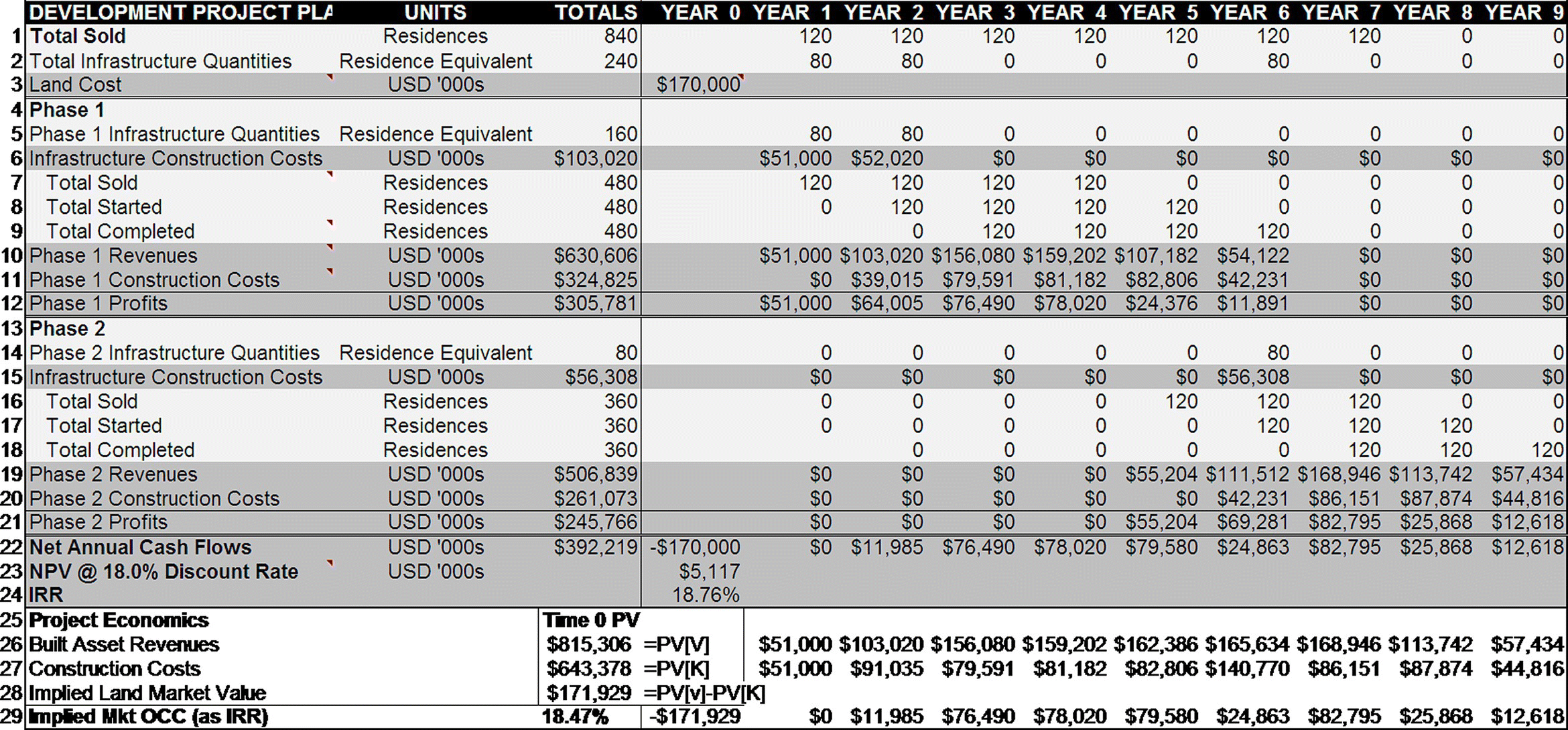
Table 22.1 presents the base plan and base case pro forma for our example project with phases. As is typical with multi‐phase projects, the pro forma shows the expected future production program and cash flows in separate parts of the table corresponding to each phase. This is the key feature that distinguishes this pro forma from those we have examined in the previous chapters. The pro forma has four sections:
- The top section (rows 1–3) is the schedule for the overall construction quantities and the upfront land cost (which we now assume is $170 M instead of the $200 M price used for the previous examples, for reasons noted in Section 22.3).
- The next two sections (rows 4–12 and 13–21) correspond to Phase 1 and Phase 2, respectively.
- The bottom section (rows 22–29) tabulates the annual net cash flow amounts for the entire project (including both phases) and the summary expected investment performance metrics. Row 23 gives the NPV net of land cost at the given 18% hurdle rate; row 24 shows the IRR at the given $170 M land price; and rows 25–29 present the project economics we describe in Section 22.3.
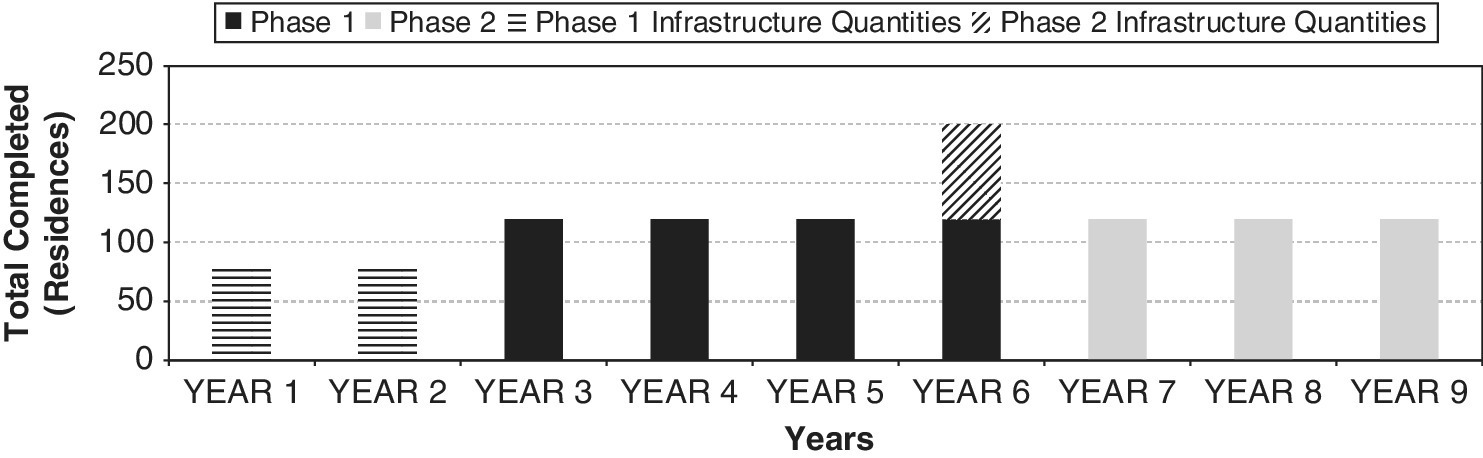
Figure 22.1a Garden City base plan: projected production, two‐phase project.

Figure 22.1b Garden City base case: projected net cash flow, two‐phase project.
Figure 22.1a shows the base plan schedule of production in bar‐chart form, and Figure 22.1b shows the base case DCF pro forma. (Compare to Figures 16.2a and 16.2b.) The two phases have the same planned production rate of 120 units per year. However:
- Phase 1 includes the two initial years of infrastructure construction, plus the first 4 years of housing construction—480 housing units altogether.
- Phase 2 includes additional infrastructure construction equal to half of the Phase 1 amount, plus another 3 years of housing construction for an additional 360 units of housing. It brings the overall project production to 840 units (marginally less than the 850 units in the Chapter 16 example project).
Phase 2 thus includes three‐quarters of the amount of housing as Phase 1, but only requires one‐half as much infrastructure. This is typical. Developers often need to front‐load more of the project’s overall necessary infrastructure in the first phase, for physical or regulatory reasons. In effect, subsequent phases can often, to some extent, “free ride” on the infrastructure of Phase 1. We assume that the investors must pay for the land entirely up front at Time 0 (and this is also when the economic opportunity cost of the land is incurred).
The base plan, Phase 2:
- Begins in Year 5 (4 years behind Phase 1) with pre‐sales of its first housing units;
- Must build its infrastructure in the following year; and
- Completes housing construction in Year 9, terminating the entire project.
This plan results in the uniform, continuous housing production seen in Figure 22.1a.
22.3 Project Economics
The NPV of this example two‐phase Garden City project differs from that of the previous example. This is because of the way the phased project spreads the rate of production over time. This results in a longer average time until receipt of revenues (or payment of costs), and thus results in lower present values of both benefits and costs. Thus:
- The gross PV of the built assets is now $815 M instead of the $883 M of the previous example project, at the same 7% OCC discount rate for these assets (see row 26 in Table 22.1).
- The PV of total construction costs also drops, to $643 M from $658 M, at the same 3% OCC discount rate that we discussed in Section 11.2 (see row 27 in Table 22.1).
- Hence, the implied value of the land is reduced to $815 M − $643 M = $172 M in the present version of the project (row 28 in Table 22.1).
If we assume that the project, as designed with the phasing proposed, is indeed providing the highest and best use of the land site, then this implies a lower bid price for the land. For simplicity, we round this to a land price of $170 M, which investors must pay entirely at Time 0.
Apart from the scaling and timing issue discussed in the preceding text, the economics and investment characteristics of the Garden City project remain much as they were in its previous versions in Chapters 16–21. The project’s overall pro forma investment risk remains very similar, as its implied market OCC of 18.47% is not very different from the 18.01% rate described in Chapter 16. (Compare the bottom row in Table 22.1 with that of Table 16.1.) This OCC reflects the amount of investment risk in the project as the capital market prices risk in the form of the implied required risk premium in the expected return. (Recall discussion in Section 11.5 and Equation 11.6.) As we noted in Section 16.5, typical practice applies a rounded hurdle rate to the traditional pro forma single‐stream net cash flow of the project. We thus retain the same 18% hurdle rate that we applied to the previous version of the Garden City project, since the investment characteristics remain essentially the same. This results in a pro forma NPV for the project of approximately $5 M at the $170 M land price, as seen in row 23 of Table 22.1 (analogous to row 20 in Table 16.1). The $170 M land price provides a pro forma going‐in IRR of 18.76% (which is not economically significantly different from the market OCC of 18.47%).
The economics of the Garden City project, as modified for phasing, are thus very similar to that of the original project described in the previous chapters. But the uniform production schedule assumed in this chapter allows us to analyze the effect of phasing delay flexibility with more generality, because the two phases are very similar.
22.4 The Delay Decision Model
As described previously, we assume that Phase 1 does not have delay flexibility; it must commence immediately in Year 1. Phase 2 must follow Phase 1 sequentially. It cannot begin at least until Year 5. But the developer can delay its start indefinitely, as long as conditions in the real estate market are not sufficiently favorable, as governed by the decision rule for delay and its input trigger value level.
The essential measure relevant for the go/no‐go decision to delay Phase 2 is the profitability implied by the pricing factors—that is, the current sales prices minus construction costs for the housing units.
The delay decision rule works as follows. In a given scenario (of the many independent random future scenarios, or trials, in the Monte Carlo simulation), in any year in which Phase 2 could otherwise start:
- If the profitability metric is below a trigger value set by the analyst, then the start of Phase 2 will be delayed for that year;
- Otherwise, Phase 2 starts in that year, and then proceeds without further delay or interruption, no matter what happens in the real estate market.
This decision rule is thus essentially the same as the Simple Myopic Delay Rule introduced in Chapter 19. Experimentation reveals that the best trigger value is the “neutral” value of zero (relative to base case profitability). This is the same result we got in Chapter 19 for the option to delay the start of the overall project (see Section 19.4 and Figure 19.6). This is not surprising, since the two options are essentially similar. In both cases, they are the possible initial delay of a production process that cannot be subsequently paused. The second phase is essentially a mini‐project by itself. The Phase 2 start delay is like an overall project start delay, except that it cannot commence right away, and it applies only to the Phase 2 part of the project. In this respect, it differs from the modular delay option we were modeling in Chapter 20, where we found that a more aggressive trigger posture was preferable.
22.5 Exploring the Value of Project Phasing Flexibility
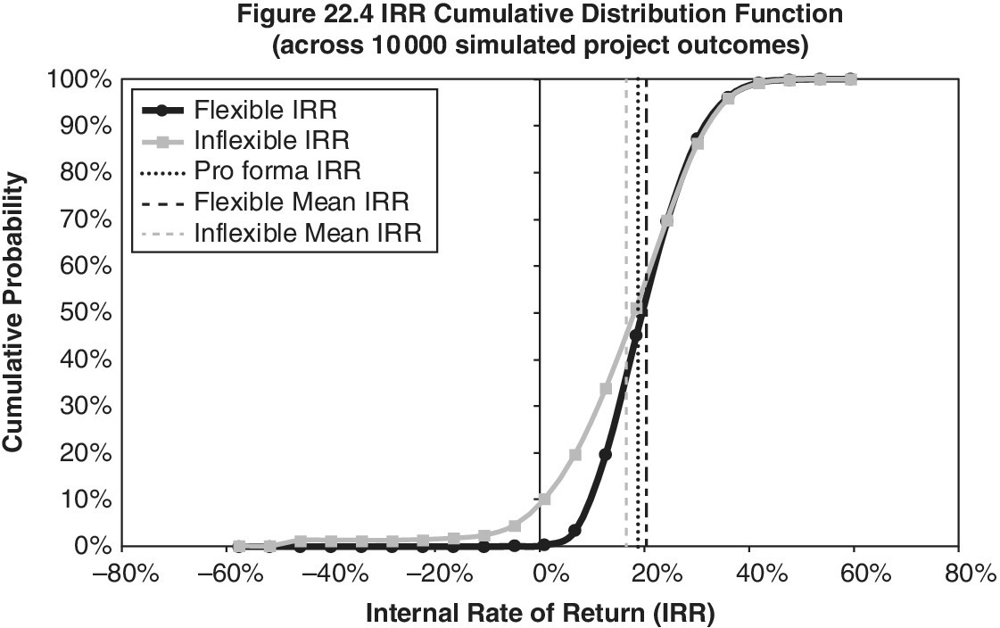
The results of the Monte Carlo simulation analysis are shown in Figures 22.2–22.5. As in the previous Monte Carlo results, the target curves represent NPV at the given project hurdle rate (18%) and the IRR at the given land price ($170 M).
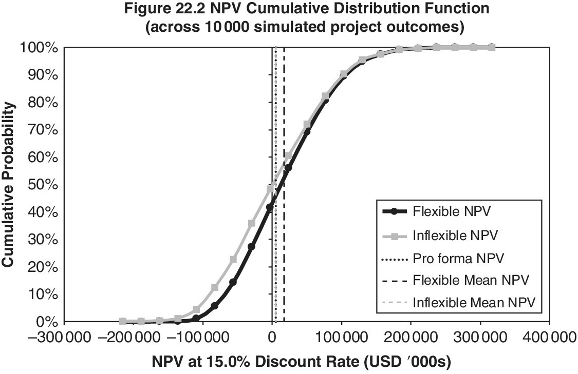


First, compare the ex‐post investment performance results recognizing uncertainty with the traditional, single‐stream pro forma NPV of $5 M (Table 22.1). The mean of the ex‐post NPV distribution in the simulation outcomes is not statistically different from the pro forma NPV. As we have seen before, this simply reflects the linearity of the present value function and the fact that our pricing factors come from probability distributions that are essentially symmetric around the pro forma pricing assumptions (that is, we assume the pro forma to be unbiased).
Next, note that the Phase 2 start‐delay flexibility provides significant value. Its ex‐post mean NPV is around $17 M, some $12 M greater than without the delay flexibility. While this gain is only about 1.5% of the pro forma gross present value of the assets to be built, it is a non‐trivial sum, and highly statistically significant. (The 95% confidence range is less than ± $0.9 M in our 10 000‐trial Monte Carlo model.) This magnitude of benefit represents 7% of the land value.
As we described in our discussion of defensive (put) options (Chapter 13), the benefit of the Phase 2 start‐delay flexibility comes from reducing the downside exposure of the project, shifting the left‐hand tail of the ex‐post performance probability distribution to the right. We can see this clearly in the sample distributions in Figures 22.2–22.5, where most of the right‐shift of the target curves for the case with flexibility occurs in the left half, well below the median performance. This is particularly true in the IRR outcome.
As before, the concavity of the IRR function causes the mean ex‐post IRR (the going‐in expected IRR) without flexibility to be slightly less than the pro forma going‐in IRR—slightly under 17% instead of closer to 19%. Additionally, the:
- Mean IRR of the flexible project averages almost 400 basis points above that of the inflexible project, at over 20% (at the $170 M land price);
- Standard deviation of the IRR outcome is reduced from almost 15% with no flexibility to less than 9% with the phase delay flexibility;
- Downside tail of the IRR distribution, represented by the 5th percentile of the outcome, exceeds that of the inflexible project by some 1300 basis points (+8% instead of −5%).
As the scatter plot in Figure 22.6 displays graphically:
- The flexible project beats the inflexible project in simulated IRR almost four times more often than the reverse happens; and
- In about 45% of the outcomes, the flexibility does not matter, as Phase 2 starts in the base plan Year 5 anyway (dots lying right on the horizontal axis).

Figure 22.6 Scatterplot of IRR outcomes for flexible versus inflexible two‐phase Garden City project.
Not surprisingly, these results are highly consistent with the quantitative results we found for the option to delay the overall project start in Chapter 19. The difference lies in the fact that the Phase 2 delay option here applies to part of the project, representing less than half its total assets, and cannot start before Year 5. Phasing delay flexibility adds non‐trivially to value, clearly improves risk/return investment performance ex‐ante, and provides important protection against severe downside outcomes that would be of particular concern to conservative investors. Also keep in mind that phasing delay flexibility will often be essentially costless—in the sense that the project owner does not need to incur any additional investment to have this sort of flexibility. It simply requires that the project be designed and planned to allow for the phasing.
Nevertheless, it is important to note that the value of the gain from the Phase 2 start‐delay flexibility is small compared to the scale of the project, and much smaller than the gains from production timing flexibility that we saw in Chapter 20 for modular flexibility. This is because delay flexibility limited to only a single subsequent phase is effectively much less flexibility than the type of general stop‐and‐restart production timing flexibility that we saw with modular production. With effectively less flexibility, we add less value.
22.6 Conclusion
This chapter focused on quantifying the value of flexibility in sequential phasing, the breakup of the overall project into distinct parts that must follow in some degree of order. Such phasing is very common in large‐scale, multi‐building projects, and it generally brings with it inherent flexibility to delay the commencement of subsequent phases (after the first). Phasing options can often be essentially “free”; you don’t have to pay anything up front to get them. You just have to plan for the phases.
This chapter walked through the process of modeling such flexibility in a spreadsheet, and then we looked at a realistic practical example, reprising our Garden City project from previous chapters (with modification). We saw that phase start‐delay flexibility adds significant value, though not nearly as much as the modular flexibility modeled in Chapter 20.