3.1 Equilibrium versus Non-Equilibrium Aging Approach

We briefly discussed equilibrium versus non-equilibrium (NE) thermodynamics damage in Section 1.3.1. Here we will use an energy approach to physics of failure problems. In NE thermodynamic degradation, we are concerned about how the aging process takes place over time so that it can be modeled. In a sense we already have one approach to this. In Chapter 2, we devised a consistent measurement process f to help measure the damage that may have occurred between times t₁ and t₂, finding the entropy damage was, as given by Equation (2.14):

(3.1)

where ΔS_f (t_i) is a quasistatic measurement. Here we can add as many intermediate quasistatic thermodynamics measurements as needed to trace out the aging path. Each measurement is taken when the system is either under very little stress or over a short enough time period, so that we are able to sample the system’s state variables over time. We then trace out how the damage is evolving over an extended time period. In this way we will be able to model the aging that is occurring by fitting the data. However, using this method we need to keep track and measure a number of states throughout the aging process. Often we are able to model the degradation (damage) so we do not have to make many measurements. In this chapter, we set the stage for NE thermodynamic damage assessment. Most of the rest of this book deals with NE thermodynamics science methods.

3.1.1 Conjugate Work and Free Energy Approach to Understanding Non-Equilibrium Thermodynamic Degradation

An approach for understanding the type of thermodynamic stresses that are occurring to the aging system is to use the conjugate work approach that we established in Section 1.4. During the quasistatic process, the work done on the system by the environment or by the system on the environment can be assessed using the conjugate variables listed in Table 1.1:

(3.2)

where we need to sum the work. If the path is well defined, we can integrate over the path from X₁ to X₂. Each generalized displacement dX_a is accompanied by a generalized conjugate force Y_a. Recall that because work is a function of how it is performed (often termed path dependent in thermodynamics), we used the symbol δW instead of dW indicating this. For a simple system there is but one displacement X accompanied by one conjugate force Y as given in Table 1.1.

We discussed how thermodynamics is an energy approach in Section 1.1 and Chapter 2. As entropy damage increases for the system, the system’s free energy decreases and the system loses its ability to do useful work (see Equation (2.131) and Figure 2.20). Then instead of focusing on entropy, we can look at the free energy of a system to understand system-level degradation. This comes down to understanding system work which we will show is one of the most important metrics for products in industry. For example, from Chapter 2 we noted that the work term for the Helmholtz free energy can be written

(3.3)

where, for simplicity, we used the conditions that . We also note that for isothermal actual work, it is bounded by the free energy . For a reversible process, the equality indicates that the free energy is the reversible work. Equation (3.3) can then be interpreted as (see also Section 2.10.4):

(3.4)

This is the thermodynamic work. Although this was obtained with simplified specific Helmholtz isothermal conditions, it can be found for the Gibbs free energy (see Chapter 5) and it proves to be relevant to many thermodynamic work processes as it is a general transparent statement. It is a statement about the free energy that equals the reversible work, as it is considered the maximum useful available work of the system.

The thermodynamic work is perhaps the most directly measurable and practical quantity to use in assessing the system’s free energy.

Therefore, we see that the actual work really characterizes the situation for many system processes. It is a good indication of the change in the system’s ability to do useful work and the damage that is created along the work path.

We can treat the initial value for the reversible work (the maximum work) prior to introducing irreversibilities as a fixed value. Then the change in actual work is some function of the change of the irreversible work over the work path:

(3.5)

Many problems in non-equilibrium thermodynamics which can be put in the category of physics of failure for semiconductors, fatigue, creep, wear, etc. come down to assessing the actual work which is dependent on the irreversible work. The irreversible work is of course dependent on the entropy damage occurring along the work path.

Therefore, in this chapter, we will explore non-equilibrium degradation processes by assessing the thermodynamic work.

3.2 Application to Cyclic Work and Cumulative Damage

In cyclic reversible work the system undergoes a process in which the initial and final system states are identical. A simple example for non-reversible cyclic work is the bending of a paper clip back and forth. The cyclic thermodynamic work is converted into heat and entropy damage in the system as dislocations are added every cycle, causing plastic deformation. This produces metal fatigue and irreversible damage, as illustrated in Figure 3.1. Aging from such fatigue is due to external forces, which eventually result in fracture of the paper clip.

If we were trying to estimate the amount of damage done each cycle, it might be more accurate to write the damage in terms of the number of dislocations produced during each cycle (see Section 2.1.1). Then we could also estimate the cumulative damage, although this number is usually unknown. We therefore take a thermodynamic approach.

For a simple system, the path in the (X, Y) plane corresponding to a cycle is shown in Figure 3.2.

The work term is . Recall that the plane can represent any one of the conjugate work variables given in Table 1.1 that can undergo cyclic work. In the (X, Y) plane, the cycle is represented by a closed curve C enclosing an area Σ. The closed curve is parameterized during the time interval of the cycle as a moving point (X(t), Y(t)) in the plane.

For a cyclic process C in a simple system, the work done on the system by the environment is given by the area obtained from the integral around a closed curve, that is:

(3.6)

The curve C representing the cycle is the boundary of an area Σ which is written here as . Employing Stokes integral theorem, one proves that the work done during a cycle may be related to the enclosed area via

(3.7)

In Figure 3.2, the system does work on the environment if the point in the plane transverses the curve in a clockwise fashion. The environment does work on the system if the point in the plane transverses the curve in a counterclockwise fashion.

A system undergoing cycles acts as an engine if the system does work on the environment during each cycle. The system acts as a refrigerator if the environment does work on the system during each cycle. In either case, during a cyclic process the system is restored to its initial state. Perhaps unfortunately, the environment is not restored to its environmental initial state after the completion of a cycle. The environment undergoes some damage during each cycle in terms of entropy in accordance with the second law of thermodynamics.

Consider a system with matter inside of automotive cylinders in a typical automobile engine. If the engine is firing on all cylinders, then the number of cycles per second would be best measured by the tachometer in terms of revolutions per minute (RPM). Before and after each cycle of motion for these cylinders, the chemical content of each cylinder will be the same (replenished). Let us say that each cycle starts with a given mixture of petroleum vapor and air inside each of the cylinders. During the cycle, the petroleum vapor and air chemically react (fuel burning) and the end-products of this chemical reaction will be belched out of the cylinders. Eventually, the noxious fumes exit the automobile through the exhaust pipe. The cylinders will move up and down exactly once during each cycle with some resulting pressure–volume cylinder work. Perhaps the environmental cylinder work (in part) slowly drags the automobile up a very annoying steep hill. A fresh new mixture of petroleum vapor and air is sucked into the cylinders at the end of each cycle, ending the completed old cycle and beginning a fresh new cycle.

A car owner might periodically ask a mechanic, in the language of American slang, “what is the damage on my automobile?” In thermodynamics we might ask, what is the damage caused to the environment during a system cycle as measured in entropy units. Here, we can discuss the notion of damage qualitatively keeping the common cyclic automobile engine example in our minds. There is damage to the environmental atmosphere when the chemical output of the fuel burning is belched out of the exhaust pipe. There is also environmental damage to the cylinders from the constant banging of the cylinder heads up and down during each cycle. Recall that the system chemical contents of a cylinder give rise to a pressure–volume work term . The cylinder wall and the cylinder head are part of the environment. The volume V inside the cylinder is an external parameter. Environmental “entropy damage” to the engine cylinder heads may get converted into the “financial damage” required for rebuilding the engine. Automobile engine failure is a typical example of the environmental entropy damage present in any real cyclic thermodynamic engine.

3.3 Cyclic Work Process, Heat Engines, and the Carnot Cycle

We typically think of an engine as a device that converts heat into motion, such as an automobile gas engine or a steam engine. We can start by considering a quasistatic cyclic process shown in Figure 3.3. The “oval” curve is an arbitrary cyclic process and the dotted lines represent a Carnot cyclic process. A Carnot cycle is often described in most thermodynamic text books because it is the most efficient heat engine that is allowed by the laws of thermodynamics. The Carnot cycle is a quasistatic operation and thus operates too slowly to be practical. However, we can use it as a good overview to illustrate the thermodynamic cyclic work and also discuss entropy damage to a heat engine.

Both cyclic processes in Figure 3.3 operate between two temperature reservoirs: the hotter reservoir of the heat source at temperature T_hot; and the colder heat sink at temperature T_cold. We have displayed it in the figure for stress–pressure and strain–volume. However, other mechanical variables can possibly be involved besides P and V, as given in Table 1.1.

The cycle consists of four quasistatic operations: (1) an isothermal expansion (i.e., constant temperature) from 1 to 2 at temperature T_hot withdrawing heat δQ_in from the source and doing work δW_in (not necessarily equal to δQ_in), where the volume expands and the pressure decreases like a piston in a car; (2) an adiabatic expansion (i.e., no heat enters or leaves) from 2 to 3, doing further work δW₂₃ but with no change in heat, ending up at temperature T_cold; and (3) isothermal compression at T_cold from 3 to 4 requiring work −δW₃₄ = δW₄₃ to be done on the system and contributing heat −δQ₃₄ = δQ₄₃ to the heat sink at temperature T_cold, ending at state 4. (4) Process 4 to 1 can be an adiabatic compression requiring work −δW₄₁ = δW₁₄ (δQ₄₁ = 0) to be done on the system to bring it back to state 1, ready for another cycle (Figure 3.3). This is a specialized sort of cycle but it is a natural one to study and one that in principle should be fairly efficient. Since the assumed heat source is at constant temperature part of the cycle must be isothermal, and if we must “dump” heat at a lower temperature we might as well give all to the lowest temperature reservoir we can find. The changes in temperature are done adiabatically.

This cycle of course does not convert all the heat withdrawn from the reservoir at T_hot into work; some of it is dumped as unused heat into the sink at T_cold. That is, more heat goes into the system than comes out:

(3.8)

For quasistatic processes, it is possible to decompose the energy change into the work plus heat differential form:

When we do work on a specific path going from an initial point to a final point, then one may write

(3.9)

Recall that we use the symbols δW and δQ as they are path dependent in exact differentials. The energy difference between the beginning and end of any process may simply be written as the difference , no matter the process between initial and final points. For a quasistatic process, it is possible to decompose an energy change into heat and work with the caveat that both the work and the heat depend on the detailed nature of the path. For a simple system, the path may be represented as a moving point (X(t), Y(t)), during the time interval of the process. For a cyclic process (closed path), one may write

(3.10)

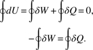
Here we have a closed system (Equation (3.10)) undergoing a cycle, so the internal energy ΔU is zero. During a quasistatic cycle, the work done by the system on the environment is equal to the total heat flow from the environment into the system. The net work done by the engine per cycle is the area inside 1234 in Figure 3.3, which is equal to:

(3.11)

The efficiency of any heat engine may be defined as the ratio of the cyclic work output to the cyclic heat input, that is:

(3.12)

Now traversing the path in Figure 3.3 in a clockwise manner, the heat is moving into the system on the top part of the cycle and out of the system on the bottom part of the cycle. We therefore find the inequalities

(3.13)

and

(3.14)

The heat moves from the environment into the system when and heat moves from the system to the environment when . However, the change in entropies ΔS_in at the hot reservoir is the same as that flowing out ΔS_out at the cold reservoir. From this relation we see that Equation (3.12) can be written as an inequality:

(3.15)

The equality yields the famous Carnot cycle efficiency:

(3.16)

We see that the efficiency of a Carnot cycle is independent of the engine and only depends on the reservoir temperature. Therefore this is totally idealized. One way of stating the second law is to say that all Carnot cycles operating between T_hot and T_cold have the same efficiencies.

If the cycle went in the counterclockwise direction, then more heat would flow out of the system than would flow into the system. For such a cycle there is net work done on the system by the environment . The system is then run as a refrigerator with efficiency . For fixed values of the maximum and minimum temperatures during a cycle, the theorem holds true for the refrigerator efficiency as well as the engine efficiency.

3.4 Example 3.1: Cyclic Engine Damage Quantified Using Efficiency

For real engines the hot section of the Carnot cycle is from 1 to 2 where heat enters into say a “working fluid,” and is then released in the Cold reservoir from 3 to 4. The temperature of the reservoir and that of the working fluid are not the same, so the process is not quite isothermal. The temperature of the hot reservoir fluid is a little cooler and the temperature of the cold reservoir fluid is a little hotter. That difference drives the efficiencies down and less work is done. For example, if the hot reservoir was at 400 K and the cold reservoir was at 200 K, the Carnot efficiency is

While the theoretical exercise of a quasistatic engine was not idealized, we can think of it as a Carnot-like engine with damage. The damage creates some inefficiency where the temperature of the fluid at the 400 K reservoir is say at 390 K and the temperature of the fluid at the 200 K cold reservoir, due to some inefficiencies, is 210 K, so that the efficiency is:

(3.17)

The actual work is of course less so the cyclic area outlined within 1234 in Area 2 of Figure 3.4 is smaller than that of the Carnot engine 1234 shown in Area 1.

One way to track cyclic engine damage is by loss of efficiency. That is, η(t) is time dependent as the engine degrades due to cyclic damage.

For a heat engine, the heat transferred into work is less and work degrades due to engine damage increase so the work out decreases with time:

(3.18)

If we compare it to a new engine, for example

(3.19)

and

(3.20)

the actual efficiency can degrade over time. The best way to quantify the loss of efficiency for any engine, not just a heat engine, is by assessing the areas in Figure 3.4. We can assess the efficiency relative to itself when the engine was new as

(3.21)

When we assess damage using this method, we must keep in mind that it is tracked over the same path as work is path dependent. If for example you were to track the efficiency of your car compared to when it was new, you could assess that by noting your miles per gallon when your car was new and compare it to when your car was older, say at 100 000 miles. To do this in a reliable way, you would need the same driving route and the same type of gas. For example, you cannot compare less-efficient city driving miles to highway miles. Further, higher-octane fuels sometimes improve engine miles per gallon (MPG) performance.

Furthermore, as we noted earlier for efficiencies in Equation (2.88), anything that adds to the irreversibility of the engine such as damage reduces our efficiency:

(3.22)

3.5 The Thermodynamic Damage Ratio Method for Tracking Degradation

In Section 2.10.4, we provided an expression for inefficiency (Equation (2.88)); this discussion was extended in Section 3.1.1. We found the reversible work is the maximum useful work that can be obtained as a system undergoes a process between two specified states as related to the free energy. The irreversibility is lost work, which is wasted work potential during the process as a result of irreversibilities. A natural use of Equation (3.3) is in assessing damage; the thermodynamic cumulative damage can be written from the sum of the inefficiencies:

(3.23)

Here we have summed the inefficiency, used Equation (3.5) and let the maximum work to failure be equal to W_rev.

This is an important deduction because it says that the damage due to the irreversibility, which is hard to measure, can be assessed from the actual work, which is easier to measure.

In terms of thermodynamic degradation in cyclic work, if we are creating damage on each cycle in the system, irreversible work damage cumulates until failure occurs. Some of the irreversibility in the total process is due to inefficiencies unrelated to system work damage. This puts a bit of reality into the difficulty in assessing the true damage. In theory we should be able to track the true system work damage as it occurs, but we should distinguish the types of damage that can be measured and/or modeled. From the above equation we will note that these inefficiencies unrelated to system work damage cancel out in the actual work assessment, so that

(3.24)

The measurable work damage ratio consists of the ratio of the actual work performed to the actual work needed to cause system failure. In system failure, we exhaust the maximum amount of useful system work. To consistently find this damage ratio, all work found must be taken over the same work path.

The path is important as there are many ways to walk up a hill; therefore, we will always require the numerator and denominator to travel the same path. For the damage expression, w_damage,i is the cyclic work damage performed over i cycles, and W_damage is the total work damage performed to cause system failure. This damage is created in the system by the environment doing work on the system, or vice versa.

In this expression we write W_total as the total actual work performed to failure and w_total,i as the total actual cyclic work performed over i cycles. As a mechanical work example, damage might be related to plastic strain; we usually can measure and/or model this.

We can now define cyclic damage over n cycles using the conjugate work variables in Table 1.1 [1, 2] as:

(3.25)

where N represents the number of cycles to failure and n represents the number of cycles prior to failure. When the damage ratio value is 1, failure results for which we require the total work summed along the path traveled in the numerator to equal the full work to failure that occurred along the same path traveled in the denominator.

In many cases it is actually possible to sum the work for each cycle in a consistent measurement process. For example, if Y is stress and X is plastic strain, we can use strain gages and monitor the stress level and integrate out the area after each cycle with computer software. An accurate estimate can therefore be made of the damage occurring. In other cases where such measurements are not possible, often what is used is the Miner’s Rule [3] that we found in Section 2.1.1. This often serves as a good approximation of the effective damage and is detailed further in Section 4.2.

If the work is non-cyclic with only one kind of work involved, and we are careful to ensure that the path traveled in the numerator is identical to that in the denominator, than the thermodynamic damage is [1, 2]:

(3.26)

If there are other types of work stress causing damage, then these can be summed as long as the work path is the same. That is, we travel up the hill on the same path but we may at times carry a different amount of weight along the way. If we travel the path with one weight we may break down just as we reach the top of the hill, while the next time we go up the path with more weight, we will break down sooner. The key is the path traveled, and then we can consider different stresses as we travel this path. Then we should be able to assess the second time up the hill if and when we will break down relative to the breakdown value of 1. In the case of other stress, we write

(3.27)

This is our approach for assessing non-equilibrium thermodynamic damage. Many examples are provided in Chapter 4.

3.6 Acceleration Factors from the Damage Ratio Principle

Reliability testing utilizes the notion of time compression to perform, say, 5 years of testing in a practical experimental time frame. The acceleration factor (AF) helps us to estimate this time compression. For example, if 1 month of testing represents 1 year in the field, then the AF is 12. AFs can be derived from first principles utilizing the thermodynamic work and the damage concept. Here we explain how this is done and, in Chapter 4, we derive from first principles numerous AFs in mechanical systems used in reliability testing. See also temperature AF in Chapter 5 and the diffusion AF in Chapter 8. In the Special Topics B section we provide application for their uses.

In NE thermodynamics, as we seek to trace the degradation process over time Equation (3.6) will often have the separable form

(3.28)

where t is time, f(Y, k, E_a) is some function of the environmental stress, and k and E_a are specific constants related to the degradation mechanism such as a specific power exponent and activation energy. Then according to Equations (3.25) and (3.26), if we have damage between two different environmental stresses Y₁ and Y₂, and failure occurs for each at time τ₁ and τ₂ respectively, then the damage value equal to 1 requires that [4]:

(3.29)

where AF_damage(1,2) is an AF used in reliability testing, often called the time compression AF between the two different stress environments 1 and 2. As an introduction to the reader who is not familiar with accelerated testing, the AF is used to estimate test time as follows:

(3.30)

Multiple examples are given in Special Topics B on AF usage, and numerous AFs are found using the damage principle in the next chapter. The concept is that, by raising the level of stress, a test can simulate life conditions over a much shorter time period. The AF is then determined by the stress equation relative to use conditions. The notation AF(test, use) then refers to the AF between test and use environments. Note that, in general, accelerating time requires AF > 1.

Then for any ith stress condition, the time to failure τ_i when AF_damage(1,i) is known is

(3.31)

When AF_damage is known, it allows us to write the damage at any time t between two stress environments along the same work path as [4]:

(3.32)

The damage AF is an important tool in assessing the time evolution of thermodynamic damage occurring between different environments. A number of AFs are derived in the next chapter. Examples of how to use the AF in testing is found in Special Topics B.

References

1. [1] Feinberg, A. and Widom, A. (2000) On thermodynamic reliability engineering. IEEE Transaction on Reliability, 49 (2), 136.
2. [2] Feinberg, A., Crow, D. (eds) (2001) Design for Reliability, M/A-COM 2000, CRC Press, Boca Raton.
3. [3] Miner, M.A. (1945) Cumulative damage in fatigue. Journal of Applied Mechanics, 12, A159–A164.
4. [4] Feinberg, A. (2015) Thermodynamic damage within physics of degradation, in The Physics of Degradation in Engineered Materials and Devices (ed J. Swingler), Momentum Press, New York.