
8
Diffusion
8.1 The Diffusion Process
Diffusion is one of the four main types of aging described in Chapter 1. Diffusion often occurs in mass-transport processes, which occur essentially from three processes: (1) convection and stirring; (2) electrical migration due to an electric field; and (3) diffusion from a concentration gradient. The first two are categorized as being under the control of an external force. This includes subtle process such as corrosion and where mass is transported in the electrolyte solution to and from the electrodes. Of these three processes, diffusion is more of a spontaneous process where external work is not involved. Diffusion can also occur in corrosion and can be a rate-controlling step. This is often the case in “hot corrosion” or “aqueous corrosion” due to oxidation. Furthermore, many aging processes due to diffusion do not involve electrochemical transitions.
For a system that is diffusing into an environment due to a concentration gradient, its energy is related to the chemical potential change. The following equilibrium thermodynamic example clarifies the important role of the chemical potential.
8.2 Example 8.1: Describing Diffusion Using Equilibrium Thermodynamics
Consider a system that can exchange energy with its environment via the diffusion process. This is shown in Figure 8.1 which as n system particles of any type in contact with an environment consisting of nenv particles of another or the same type. The particles could be atoms, ion, or molecules representing a chemical species of interest.
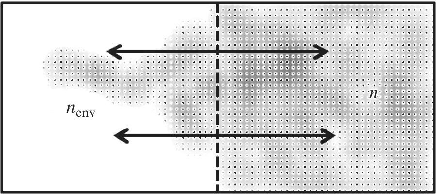
Figure 8.1 System with n particles and nenv environment particles
We can make an analogy to Example 2.10. Following a similar treatment, the spontaneous diffusion process seeks to maximize
The subscript env is for “environment” and we are not using a subscript here for the system. The system can exchange energy and atoms with the environment subject to the constraint of energy and particle conservation. The total conserved energy is
and particle number is
For a closed process this obeys
The entropy for the system and environment requires
Then we can write from the combined first and second law equation using the work conjugate pair for the chemical potential in Table 1.1 (also see Section 5.2):

or, equivalently from Equations (8.4) and (8.5), ![]() and
and ![]() yielding
yielding

In order to ensure that the total entropy goes to a maximum, we have positive increments under the exchange of energy and matter in which the system energy change is dU. If the system’s chemical potential is greater than the environment’s chemical potential, that is,![]() , then this dictates that
, then this dictates that ![]() and particles are diffusing out of the system side to the environment. If the system’s chemical potential is less than the environment’s chemical potential, that is,
and particles are diffusing out of the system side to the environment. If the system’s chemical potential is less than the environment’s chemical potential, that is, ![]() , then this dictates that
, then this dictates that ![]() . The particles are increasing in the system. The particles will then flow from the higher-chemical-potential region to the lower-chemical-potential region, similar to the potential of a battery.
. The particles are increasing in the system. The particles will then flow from the higher-chemical-potential region to the lower-chemical-potential region, similar to the potential of a battery.
If entropy is at the maximum value, then the first-order differential equation vanishes. Therefore, for equilibrium when the entropy is maximum T = Tenv and ![]() , so that
, so that ![]() . As well the pressure (P = nRT/V) is the same in the system and environmental regions at equilibrium in Figure 8.1 as the particles mix. Particles therefore migrate in order to remove differences in chemical potential. Diffusion ceases at equilibrium when
. As well the pressure (P = nRT/V) is the same in the system and environmental regions at equilibrium in Figure 8.1 as the particles mix. Particles therefore migrate in order to remove differences in chemical potential. Diffusion ceases at equilibrium when ![]() . The statement that diffusion occurs from an area of high chemical potential to low chemical potential is the same as saying that the diffusion process occurs from an area of high concentration to an area of low concentration. While this diffusion flow is a natural spontaneous process, the opposite cannot occur. That is, in accordance with the entropy maximum principle in Chapter 1, we see that the reveres process cannot occur without some work. The particles will not separate back once they are mixed without some amount of work done to accomplish this.
. The statement that diffusion occurs from an area of high chemical potential to low chemical potential is the same as saying that the diffusion process occurs from an area of high concentration to an area of low concentration. While this diffusion flow is a natural spontaneous process, the opposite cannot occur. That is, in accordance with the entropy maximum principle in Chapter 1, we see that the reveres process cannot occur without some work. The particles will not separate back once they are mixed without some amount of work done to accomplish this.
In a manner of speaking, the diffusion process has degraded so that no spontaneous energy exchange occurs and the system is in its lowest free energy state or maximum entropy state with the environment. Of course, we can have a quasistatic equilibrium condition when the diffusion process is fully concentrated and negligible particle exchange is occurring.
8.3 Describing Diffusion Using Probability
Diffusion can also be understood using a probability approach. Consider particles such as impurities; these impurities distribute themselves in space with passing time. For example, in semiconductors impurities deposited in optimal regions in space later diffuse to undesirable regions as the semiconductor ages. Raising the temperature may accelerate such aging.
To describe diffusion using probability, the Central Limit Theorem (Figure 8.2) is sometimes useful (see Special Topics A6). For example, the theorem applies for systems subject to a large number of small independent random effects as in a random walk (see Section 2.8.1). The central limit theorem is used in the sense that if we have X1, X2,…, XN identically distributed random clusters of particles, each with a mean and variance, then the average of the entire system will approach a normal distribution as N approaches a large quantity of particles, moving as in a random walk manner. Here impurity particles are concentrated in a small region, each with an irregular random walk motion. From the Central Limit Theorem, the positions will become normally distributed in space for times short on a macroscopic scale but long on a microscopic scale. In one dimension, the distribution after time t will appear to be Gaussian.
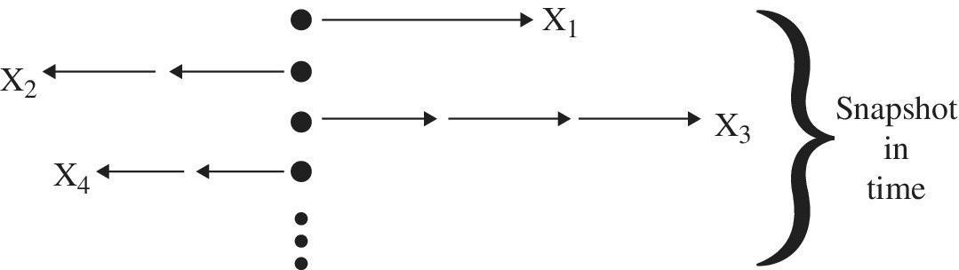
Figure 8.2 Diffusion concept
Therefore, the probability P of finding a particle a distance x from the point of initial highest concentration taken as the origin, where one can center the mean (as in Figure 8.2), is

In diffusion theory for this typical physical situation it is found that the particles spread linearly with time (t) with the variance as
The proportionality constant is the diffusion coefficient D times 2 [1]:
(Note that σ has the same units as meter and D has units of square meter per second.)
The probability of finding a particle at position x from the origin at time t in one-dimension is then

In terms of our semiconductor problem, if Q were the number of impurity particles in a unit area and C is the concentration of these impurities in the volume, the concentration distribution can be written

The result is the solution to the diffusion equation with the boundary conditions for a physical situation described above. In one dimension, the diffusion equation that this satisfies is
The reader may be interested to show that the solution above satisfies this diffusion equation by direct substitution of Equation (8.14) into (8.15). It is important to note that the solution obtained is subject to the correct initial conditions.
8.4 Diffusion Acceleration Factor with and without Temperature Dependence
The diffusion coefficient itself is found to have Arrhenius temperature dependence

where Δ is the barrier height (see Section 6.1). As T increases so does D (with an Arrhenius form). Note that since D occurs only as a product Dt (Equation (8.12)), the time scale is effectively changed (accelerating time) with an Arrhenius temperature dependence.
The diffusion acceleration factor will vary according to the diffusion rate ratio
where AFT is given earlier in Equation (5.20) and AFx is the acceleration factor due to spatial concentration gradient, defined:

8.5 Diffusion Entropy Damage
When describing diffusion using probability theory, we noted that the variance is a key intensive variable. Therefore, we anticipate entropy damage to be dominated by the variance. Diffusion is a continuous intensive variable of the system. In terms of degradation, we will consider that an increase in diffusion degrades the system of interest over time.
In Chapter 2 we noted that the entropy of a continuous variable is treated in thermodynamics using the concept of differential entropy which, for continuous variables as in the diffusion case, is
Now we have treated the particle distribution in the diffusion process as Gaussian. We then found from this function that the differential entropy results were given by (see Chapter 2, Equation (2.35))
This key result can be applied to the diffusion process here. We see that for entropy for a Gaussian diffusion system, the differential entropy is only a function of its variance σ2 (independent from its mean μ). For a system that is diffusing over time, the entropy damage can then be measured in a number of ways where the change in the entropy at two different times t2 and t1 is

Substituting from Equation (8.12), ![]() , we write
, we write

where we assume ![]() . Therefore, entropy diffusion damage at a constant temperature, due to a concentration spatial gradient that is Gaussian, apparently occurs as logarithmic in time in this view.
. Therefore, entropy diffusion damage at a constant temperature, due to a concentration spatial gradient that is Gaussian, apparently occurs as logarithmic in time in this view.
This is an important result and actually agrees with previous theory that was presented in the thermally activated time-dependent (TAT) model (Chapters 6 and 7). There we found that a number of processes were described as aging in log time for thermally activated processes. Many natural aging processes have been observed to age with log(time) such as transistor degradation, crystal frequency drift, and early stages of creep. In fact, diffusion can play a role in degradation such as transistor aging (junction doping issues), intermetallic growth, contamination issues, and so forth. This result provides insight for the TAT model and these physical natural aging processes. Many complex aging processes can have a rate-controlling diffusion mechanism.
8.5.1 Example 8.2: Package Moisture Diffusion
A +85°C and 85% relative humidity (%RH) test is performed on a plastic molded semiconductor device. It is of interest to estimate how long it takes for the moisture to penetrate the mold and reach the die. We can estimate this time using the diffusion expression above. We use the experimentally reported values of:
where L is the molding compound thickness of 0.05 inches; ![]() for moisture penetration into the mold; and
for moisture penetration into the mold; and ![]() .
.
Solving the diffusion expression above (Equations (8.12) and (8.16)) with the time-dependent variance for t yields

As a side note, this process does not appear at first to be a logarithmic-in-time model as might be suggested by Equation (8.22). However, we could first rearrange the above equation in terms of the following time-dependent power law

We have noted in Section 6.2.1 (see Figure 6.3) that power laws of the form tk where 0 < k < 1 can be modeled with a log(time) form (see Equations (6.9) and (6.10)). That is, through proper modeling we anticipate that a TAT model can be found for this thermally activated process, in the form
that would equally model the physics of the situation.
Now Equation (8.24) is in terms of R, the gas constant. It is instructive and simplest to put the exponential function in terms of Boltzmann’s constant. Boltzmann’s constant is by definition kB = R/NA. To put the expression in terms of Boltzmann’s constant, one would divide through the exponential expression by Avogadro’s number (NA = 6 × 1026 molecules/mole).

Now ![]() . Inserting the numbers into the above expression yields
. Inserting the numbers into the above expression yields

8.6 General Form of the Diffusion Equation
The most generalized diffusion equation for aging circumstances can include external forces, such as an electric field. For example, if the flux is a charged species and is driven by a force such as a constant electric field E, then [1]
Note that this equation shows that the diffusion equation can describe all three processes that we have categorized as fundamental to aging in Section 1.2: a thermally activated Arrhenius process with D(T) dependence; the existence of a spatial gradation driving diffusion; and an external forced process. All processes are fundamentally driven by the thermodynamic state. The equation would be extremely difficult to solve if all mechanisms were equally important. However, aging can often be separated into its rate-controlling processes.
Reference
- [1] Morse, P.M. (1969) Thermal Physics, Benjamin/Cummings Publishing, New York.