
4.1
Construction of the Real Numbers
4.1.1 Introduction
No doubt, most readers of this book think of real numbers as values on a number line, which has long been accepted by scientists and engineers as a model for measurements of length, mass, and time.
Although there is nothing wrong with this intuitive interpretation, it is the goal of this section to show how the real numbers can be logically created from more primitive number systems like the natural numbers, as well as introducing aspects of the real numbers decimal expansions, the least upper bound property, types of real numbers like rational, irrational, algebraic, and transcendental, and completeness properties.
Without going into the history of how numbers went from 1, 2, 3, … to the real numbers, there are two fundamental approaches to how to define the real numbers. First, we can state axioms that we believe characterize our interpretation of the real numbers. This is the here they are, the real numbers. This approach is called the synthetic approach, whereby axioms hopefully embody what we believe a “continuum” should be.
On the other hand, we can “construct” the real numbers, much like a carpenter builds a house. In this approach, we begin with what our distant ancestors gave us, the natural numbers 1, 2, 3, …. We then take these numbers and doing some “mathematical carpentry” replacing hammers and nails with a little set theory and predicate logic, to logically construct, step‐by‐step, the real numbers. This is the approach taken in this section, starting with the natural numbers we construct the integers, then the rational numbers, all the way to real numbers. The synthetic axiomatic approach of here they are will be left to the next section.
4.1.2 The Building of the Real Numbers
The construction of the real numbers begins with the simplest numbers, the natural numbers
then, by a series of steps we construct the integers
followed by the rational numbers
and finally, the real numbers ℝ.
4.1.3 Construction of the Integers: ℕ → ℤ
The way we construct the integers 0, ± 1, ± 2, … from the natural numbers 1, 2, 3, … is to define integers as pairs of nonnegative integers, where we interpret each pair (m, n) as the difference m − n. Thus, the pair (2, 5) of natural numbers is defined as −3, the pair (7, 1) as 6, and the pair (4, 4) as zero. If we then define addition, subtraction, and multiplication of these pairs (m, n) consistent with the arithmetic of the natural numbers, we have successfully defined the integers in terms of the natural numbers.
To carry out this program, we begin with the Cartesian product
of pairs of natural numbers, called grid points, which are illustrated in Figure 4.1.
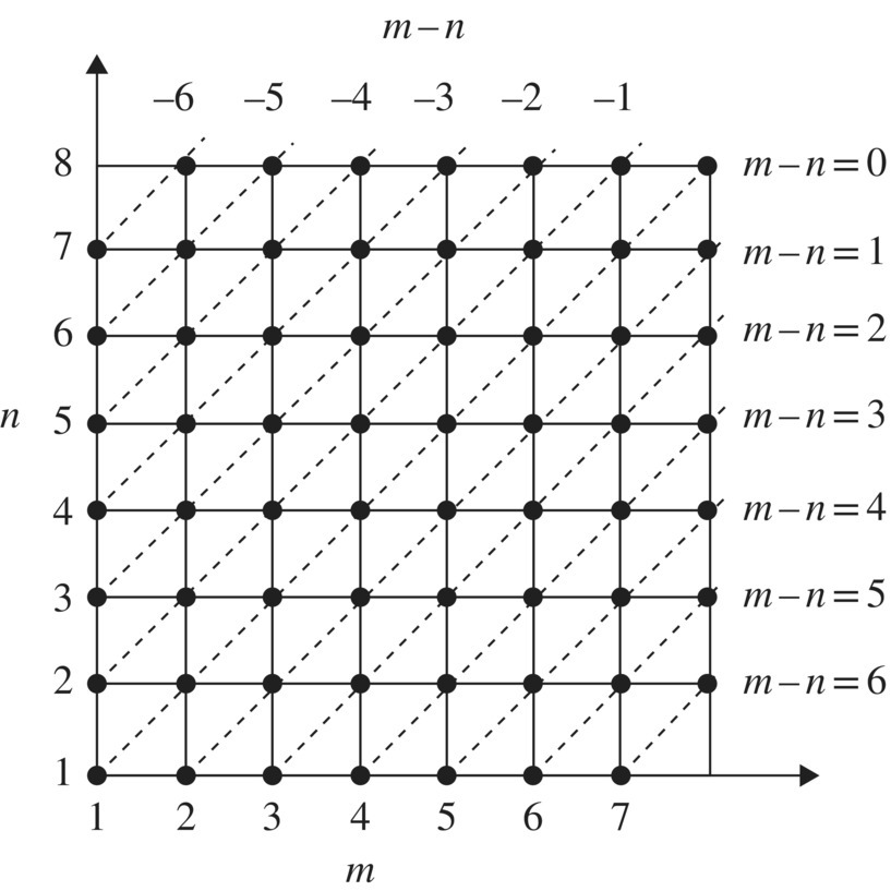
Figure 4.1 Partitioning ℕ × ℕ into equivalence classes.
We now define an equivalence relation “≡” between pairs of natural numbers by
This relation can easily be verified to be an equivalence relation and its verification is left to the reader. See Problem 1. We saw in Section 3.3 that equivalence relations on a given set partitions the set into disjoint equivalence classes. In this case, the equivalence classes consist of grid points on 45° lines as drawn in Figure 4.1. A few of these equivalence classes are listed in Table 4.1, designated by ![]() which shows a representative member of each equivalence class. Each one of these equivalence classes will define an integer. For example, the equivalence class
which shows a representative member of each equivalence class. Each one of these equivalence classes will define an integer. For example, the equivalence class ![]() defines zero,
defines zero, ![]() defines −1,
defines −1, ![]() defines +1.
defines +1.
Table 4.1 Five equivalence classes.
| Equivalence class | Integer definition |
| −2 | |
| −1 | |
| 0 | |
| 1 | |
| 2 |
We now define the integers ℤ as the collection of all these equivalences classes. In other words
which we write as
We can also define the nonnegative and negative integers as

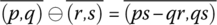
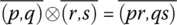
We now must define addition, subtraction, and multiplication for the integers, consistent with the rules of the natural numbers. We define for p, q, r, s ∈ ℕ addition ⊕, subtraction ⊖, and multiplication ⊗ of integers (represented by pairs of natural numbers) by:
- Addition:
- Subtraction:

- Multiplication:

For example
- Addition:

- Subtraction:

- Multiplication:

When p > r and q > s, the pairs (p, r) and (q, s) correspond to p − q > 0 and r − s > 0, hence, the above definition of addition, subtraction, and multiplication of pairs of natural numbers reduces to identities of the natural numbers.
4.1.4 Construction of the Rationals: ℤ → ℚ
We now move up the number chain and construct the rational numbers ℚ from the integers ℤ using a strategy similar to what we did in constructing the integers as pairs of natural numbers.
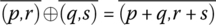
To carry this out, define an equivalence relation on ℤ × (ℤ − {0}) by
where (m, n) and (m′, n′) are pairs of integers and we “interpret” them as m/n and m′/n′, respectively. This equivalence relation partitions the grid points in ℤ × (ℤ − {0}) into distinct equivalence classes as drawn in Figure 4.2. Observing the following equivalences
we see that the equivalence classes consist of the grid points on straight‐lines passing through the origin, where the equivalence class with representative (m, n) is assigned the rational number m/n. For example
Figure 4.2 Equivalence classes defining rational numbers.
A few equivalence classes with an arbitrary designated representative are shown in Table 4.2.
Table 4.2 Five equivalence classes in ℤ × (ℤ − {0}).
| Equivalence class | Rational correspondence |
| −1 | |
| 0 |
We now define the rational number p/q as
We now define the arithmetic operations on the newly formed rational numbers.
- Addition:
- Subtraction:
- Multiplication:
For example
- Addition:

- Subtraction:

4.1.5 How to Define Real Numbers
We now come to a fork in the road. There are several ways to define the real numbers and each has its merits and demerits. On the one hand, we could define real numbers in the way they were described to you in grade school, as decimal expansions. This is nice since all numbers, rational and irrational are more or less treated in the same way, and we normally perform arithmetic when numbers are written in this form, like 2.35 + 4.91. However, on the negative side, when real numbers are represented by expressions of the form
where the as and bs are decimal digits, it is the dot, dot, dot at the end of the expansion that causes problems theoretically. Another problem is that certain real numbers have more than one decimal expansion, like
Like we said, there is that nasty dot, dot, dot again.
Still another demerit for the decimal expansion interpretation of real numbers is that they do not relate visually to points on a continuous number line, which is how most people like to think of real numbers.
However, there are two more approaches for defining the real numbers, one due to Cantor and the other due to his close friend Richard Dedekind. Both of these approaches are based on defining the real numbers in terms of the rational numbers, much like we defined the rational numbers in terms of the integers. Cantor's approach defines real numbers limits of sequences of rational numbers, like in the definition of the irrational real number π being the limit of the sequence
Although this approach has intuitive appeal, it demands that the reader develop a background in sequences, convergence, null sequences, and other concepts from real analysis, not introduced in this book. Hence, we follow the second approach, that due to Richard Dedekind.
Although rational numbers have many desirable properties, they have from the perspective of calculus, the undesirable property that they have “gaps” like the gaps at ![]() and π. In fact, there are an infinite number of gaps, and as we have seen in Section 2.5, an uncountable number of gaps. The idea is to “fill in” these gaps, and arriving at a new number system called the real numbers.
and π. In fact, there are an infinite number of gaps, and as we have seen in Section 2.5, an uncountable number of gaps. The idea is to “fill in” these gaps, and arriving at a new number system called the real numbers.
4.1.6 How Dedekind Cuts Define the Real Numbers
Dedekind's 1872 idea appeals to our intuitive grasp of the rational numbers aligned on a line. His idea was to partition the rational numbers into two disjoint sets L and U satisfying the following two conditions.
The above definition of a Dedekind cut does not uniquely define a partition of the rational numbers, but three different partitions called Dedekind cuts. They are as follows.

Figure 4.3 Type 1 Dedekind cut.
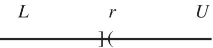
Figure 4.4 Type 2 Dedekind cut.
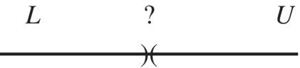
Figure 4.5 Type 3 Dedekind cut.
Each Dedekind cut of Type 1 or Type 2 corresponds to a rational number, whereas a Dedekind cut of Type 3 correspond to a number that is not rational. These are numbers that fill all the gaps between rational numbers. These are called irrational numbers. This leads us to the Dedekind cut definition of the real numbers.

Figure 4.6 Dedekind cuts for 2 and  .
.
4.1.7 Arithmetic of the Real Numbers
Now that we have defined the real numbers, the next job is to Dedekind cuts to define addition, subtraction, multiplication, and division of the real numbers (as well as defining order relations like < and ≤) consistent with those of the rational numbers. Although we can define arithmetic operations of real numbers in this way, they are rather complicated, and we will not include them here. If we had to carry out even the easiest arithmetic, like adding ![]() using the Dedekind cut definition, it would a difficult task. As we all know, the way we do arithmetic involving irrational numbers, we replace them by a decimal digits,
using the Dedekind cut definition, it would a difficult task. As we all know, the way we do arithmetic involving irrational numbers, we replace them by a decimal digits, ![]() and find the approximate value
and find the approximate value ![]() . Of course, we cannot be 100% accurate like we are when we restrict arithmetic to the rational numbers, like
. Of course, we cannot be 100% accurate like we are when we restrict arithmetic to the rational numbers, like
but that is the price of enlarging our number system to the real numbers.
Problems
- Equivalence Relation I
Show that the relation ≡ on ℕ defined by

between pairs of natural numbers (m, n) and (m′, n′) is an equivalence relation.
- Equivalence Relation II
Show that the relation ≡ on ℤ defined by

between pairs of integers (m, n) and (m′, n′) is an equivalence relation.
- Arithmetic in ℤ
We defined the integers ℤ in terms of pairs of natural numbers (m, n) belonging to an equivalence class. Perform the following arithmetic for integers as defined in the book. What does each operation represent in the language of integers?
- d e f Arithmetic in ℚ
We defined the rational numbers ℚ in terms of pairs of integers (m, n) belonging to an equivalence class. Perform the following arithmetic for rational numbers using the definition in the book. What does each operation represent in the language of rational numbers?
- d

- e
- f

- d
- Decimal to Fractions
Find the fraction for each of the following real numbers in decimal form, where the bar over numbers means the numbers are repeated.
- 0.9999….

- 0.232 323 23….

- 0.012 312 312 3….

- 0.001 111….

- 0.9999….
- Two Decimal Representations
The real numbers that have two different decimal representations agree up to some point, but then one continues with a999…, while the other continues with b000…, where the digit a is one more than the digit b. The dot, dot, dot at the end of the expression refers to a never‐ending list of digits. Write several instances of real numbers that have two decimal representations.
- Irrationals Everywhere
Show that between any two rational numbers, there is an irrational number. Hint: For two rational numbers r1 < r2, there exists a natural number n that satisfies
 . Using this inequality, we can construct a number between r1 and r2. The only remaining task is to show this number is irrational.
 - Rationals Everywhere
Show that between every two irrational numbers there is a rational number. Hint: Let i1 and i2 be two irrational numbers with i1 < i2. Hence, there exists a natural number n satisfying
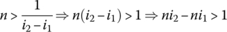
Use the last result to construct a rational number m/n that lies between i1 and i2.
- Internet Research
There is a wealth of information related to topics introduced in this section just waiting for curious minds. Try aiming your favorite search engine toward construction of the integers from the natural numbers, construction of the rational numbers from the integers, Dedekind cut, and Richard Dedekind.