
4.2
The Complete Ordered Field: The Real Numbers
4.2.1 Introduction
Advances in function theory in the nineteenth century demanded a deeper understanding of the real numbers, which led to a “rigorization” of analysis by such mathematical greats as Cauchy, Abel, Dedekind, Dirichlet, Weierstrass, Bolzano, Frege, Cantor, and others. A deeper understanding of functions required precise proofs which in turn required the real number system be placed on solid mathematical ground.
Although we generally think of real numbers as points on a continuous line that extends endlessly in both directions, the goal of this chapter is to strip away everything you know about the real numbers and start afresh. This is not easy since all knowledge and mental imagery of the real numbers created over a lifetime is firmly entrenched in our minds. But if the reader is willing to wipe the slate clean and start anew, we will introduce you to a new mathematical entity, known by mathematicians as the complete, ordered field, which, for lack of another name, we call ℝ. By building the axioms of the real numbers, you will have a deeper understanding of them than simply as “points on a very long line.”
There are three types of axioms required to define the real numbers. First, there are the arithmetic axioms, called the field axioms, which provide the rules for adding, subtracting, multiplying and dividing. Second, there are the order axioms, which allow us to compare sizes of real numbers like 2 < 3, 4 > 0, and −3 < 0, and so on. And last, there is an axiom, called the completeness axiom, which gives the real numbers that special quality which allows us to think of real numbers as “flowing” continuously with no gaps.
So let us begin our quest to define the holy grail of real analysis.
4.2.2 Arithmetic Axioms for Real Numbers
We begin by defining a set ℝ, but do not think of ℝ as the real numbers yet. We begin by defining two binary functions from ℝ × ℝ → ℝ, one called the addition function and the multiplication function. The addition function assigns to each pair (a, b) of numbers in ℝ a new element of ℝ called the sum of a and b and denoted by a + b. The multiplication function assigns to each pair of elements in ℝ a new element in ℝ called the product of a and b and denoted by a × b or more often simply ab. These operations are called closed operations since when a, b ∈ ℝ so are a + b and ab.
These axioms have passed the test of time and are now chiseled in stone in the laws of mathematics and form an algebraic system called a field1(or an algebraic field), which is summarized as follows.
4.2.3 Conventions and Notation
In addition to the above axioms, we make the following conventions;
- The associative axioms for both addition and multiplication tell us it does not matter where the parentheses are placed. In other words, we can write a + b + c for a + (b + c) or (a + b) + c. The same associative law holds for multiplication, which allows us to write abc = a(bc) = (ab)c.
- The unique additive inverse of an element a is denoted by −a. Hence, we have a + (−a) = 0. The multiplicative inverse of a is denoted by a−1 and often written 1/a. Hence, aa−1 = a (1/a) = 1.
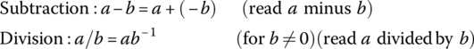
Two other operations of subtraction and division can be defined directly from addition and multiplication by
We know what you are thinking: you have known all this since third−grade. If your argument is that the axioms of arithmetic are simple and elementary, that is no argument at all. Axioms are supposed to be simple and elementary. The question you should ask is what kind of results can be proven from the axioms. The answer is an algebraic field can give rise to many deep results. Ask yourself if these are the simplest axioms that give rise to a system of arithmetic? Do you need any more axioms? Can you get by with less? These are not trivial questions and their answers are even less so. There are other systems of axioms that allow you to perform “arithmetic” operations on elements of a set, such as groups and rings that we will learn about in Chapter 6 when we study abstract algebra.
4.2.4 Fields Other than ℝ
- Boolean Field: Let F2 = {0, 1} and define the binary operations of addition and multiplication by Table 4.4.
The set A with these arithmetic operations is an algebraic field. We leave it to the reader to check all the properties a field must possess.
- Complex Numbers: The complex numbers a + bi, where a, b are real numbers and
 , where addition and multiplication are defined in the usual manner.
 - Rational Numbers ℚ: The rational numbers where addition and multiplication are defined in the usual way.
- Rational Functions F: The set of all rational functions

where p(x), q(x) ≠ 0 are polynomials with real coefficients, where addition and multiplication are defined in the usual way and 0 and 1 are the standard additive and multiplicative identities.
| Field axioms | |
| A field is a set, which we call ℝ, with two binary operations, called + and ×, where for all a, b and c in ℝ, the following axioms hold.a | |
| Addition axioms | Name of axiom |
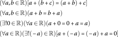 |
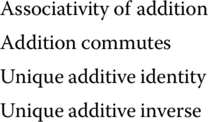 |
| Multiplication axioms b | Name of axiom |
 |
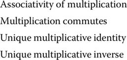 |
| Distributive axiom | Name of axiom |
| (∀a, b, c ∈ ℝ)[a(b + c) = ab + ac] | Multiplication distributes over addition |
a We call the field ℝ since we are concentrating on the real numbers, but keep in mind there are many examples of an algebraic field. It is assumed in the axioms for a field that the additive identity 0 and the multiplicative identity 1 are not equal.
b We often drop the multiplication symbol “·” and denote multiplication of two elements as a ⋅ b = ab.
Table 4.4 Boolean field.
| + | 0 | 1 | × | 0 | 1 | |
| 0 | 0 | 1 | 0 | 0 | 0 | |
| 1 | 1 | 0 | 1 | 0 | 1 |
There are many other examples of fields studied by mathematicians, including the Galois finite fields, p‐adic number fields, and fields of functions, such as meromorphic and entire functions.
We now come to the second group of the three types of axioms required to describe the real numbers.
4.2.5 Ordered Fields
Although an algebraic field allows us to carry out arithmetic on a set, what it cannot do is compare sizes of members of the set. The job now is to include “order” on the field. To do this, we split the field into two disjoint sets, P and N, called the negative and positive members of the field. These two sets mimic the properties of the positive and negative real numbers. This motivates the general definition of an ordered (algebraic) field.
4.2.6 The Completeness Axiom
If we were to stop with ordered fields, we would be neglecting that special ingredient that defines the real numbers as a continuum. There are many examples of ordered fields that are not the real numbers, and all those algebraic systems have “gaps” between their elements. The set of rational numbers is an ordered field, which as we all know, has an uncountable number of gaps between its members, two gaps being the solutions of x2 = 2, which are ![]() , which was proven long ago to be not a rational number. What we need is an axiom that “fills in” these gaps and this is where the completeness (or continuum) axiom comes into play.
, which was proven long ago to be not a rational number. What we need is an axiom that “fills in” these gaps and this is where the completeness (or continuum) axiom comes into play.
An interesting aspect of this axiom is that over the years mathematicians have found several completeness axioms that are logically equivalent. Thus, it is possible to introduce any one of them as the “completeness” axiom. In this book, we have chosen the “version” of the completeness axiom as the least upper bound axiom, our reason being many interesting concepts can be deduced by working with it. Then, there is the other benefit, it is easy to understand. Before stating the axiom, however, we review a few important ideas about the least upper bound of a set introduced in Section 3.2.
4.2.7 Least Upper Bound and Greatest Lower Bounds
We use the four intervals in Figure 4.7 as a prop for reviewing the concepts of the least upper bound (lub) and the greatest lower bound (glb) introduced in our study of orders in Section 3.2.
Figure 4.7 Max, min, lub, glb.
The intervals (a, b), [a, b], [a, b), and (a, b] are all bounded, both above and below. Bounded above simply means there is at least one number greater than or equal to the elements in the set. Likewise, a lower bound for a set is a number less than or equal to the elements in the set. Of course, not all sets are bounded; the set [1, ∞) is bounded below but not above, and (−∞ , ∞) is bounded neither above nor below. The intervals [a, b] and (a, b] each have a maximum value of b, whereas the intervals (a, b) and [a, b) do not have a maximum value. The same arguments hold for minimum values. The intervals [a, b], [a, b) each has a minimum value of a, but the intervals (a, b) or (a, b] do not have minimum values.
So what is the meaning lub (A) and glb (A) in Figure 4.7? Note that two of the intervals contain their maximum value and two do not. However, and this is the important part, for each of the four intervals [a, b], [a, b), (a, b), and (a, b], the set of upper bounds is the same, namely [b, ∞), and note that this set of upper bounds contains its minimum of b. For the intervals (a, b), [a, b) where b does not belong to the interval, we call b the least upper bound (or supremum) of the set since it is the least of the upper bounds of the set. We denote this value by lub(A). For the two sets [a, b] and (a, b] that have a maximum value, the least upper bound of the set is the same as the maximum of the set. For the sets (a, b) and [a, b) that do not have maximum values, the least upper bound b is a kind of “surrogate” for the maximum.
The same principle holds for lower bounds. The set of lower bounds for the four intervals is the same, namely (−∞, a]. The number a is the greatest of all these lower bounds and is called the glb(A) for each of the four intervals. Any set that is bounded below may or may not have a minimum value, but the set of lower bounds will always have a maximum value, and that maximum value is called the greatest lower bound (or infimum) of the set and denoted by glb(A).
Figure 4.8 Least upper bound.
Figure 4.9 Greatest lower bound.
This leads us to the completeness axiom for ℝ, which up to now, we endowed with only field and order axioms. The last set of axioms we assign to ℝ (actually only one axiom) is called the completeness axiom.
We are now (finally) ready to define the real numbers.
The least upper bound axiom is necessary since there are ordered fields that do not “look like” the real numbers and the reason is that they do not satisfy the least upper bound axiom. Of the ordered fields that do not satisfy the completeness axiom, the rational numbers are the most well‐known. By including the completeness axiom with an ordered field, the ordered field behaves like the real numbers.
When we refer to the real numbers as a complete ordered field, we always say the complete ordered field since all complete ordered fields are isomorphic. We say that two abstract structures are isomorphic if they have exactly the same mathematical structure and differ only in the symbols used to represent various objects and operations in the system.
Problems
- True or False
- The natural numbers ℕ with operations of addition and multiplication is an ordered field.
- ℚ and ℝ are ordered fields but ℂ is not.
- For A, B bounded sets of real numbers, the identity

holds, where A − B = {a − b : a ∈ A, b ∈ B}.
- The integers ℤ constitute an ordered field.
- All finite sets of real numbers have a least upper bound.
- The rational numbers less than 1 have a least upper bound.
- If a subset of the real numbers has an upper bound, then it has exactly one least upper bound.
- sup(ℤ) = ∞
- Every finite set can be ordered.
- The set of linear functions f(x) = ax + b with the usual addition and multiplication of functions is an algebraic field.
- In plain English, the completeness axiom ensures there are no “holes” in the real numbers.
- Solving a Middle School Equation
Show that (∀a, b ∈ ℝ) the equation a + x = b has exactly one solution, which is x = b + (−a).
- Glb, Lub, Max, and Min
If they exist, find max(A), min(A), lub(A), and glb(A) for the following sets.
- A = {1, 3, 9, 4, 0}
- A = [0, ∞)
- A = {x ∈ ℚ : 0 ≤ x < 1}
- A = [−1, 3]
- A = {x : x2 − 1 = 0}
- A = {n ∈ ℕ : n divides 100}
- A = {x ∈ ℝ : x2 < 2}
- A = (− ∞ , ∞)

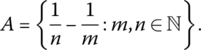
- More Difficult Sup and Inf
If they exist, find the least upper bound and greatest lower bound of the set
- Algebraic Field
Show that the rational numbers with the operations of addition and multiplication form an algebraic field.
- Boolean Field
Show that the set F2 = {0, 1 } consisting of two elements and following arithmetic operations forms an algebraic field as shown in Table 4.5.
- Ordered Field
Show that the rational numbers with the operations of addition and multiplication and usual ordering relation “less than” “<” form an ordered field.
- Not an Ordered Field
Show that the complex numbers is an algebraic field but not an ordered field.
- Well‐Ordering Principle
The well‐ordering principle3 states that every (nonempty) subset A ⊆ ℕ contains a smallest element under the usual ordering ≤. Does this principle hold for all subsets A ⊆ ℤ?
- Well‐Ordering Theorem
A partial order “
 ” on a set X is called a well‐ordering (and the set X is called well‐ordered) if every nonempty subset S ⊆ X has a least element. The Well‐Ordering Theorem4 states that every set can be well‐ordered by some partial order. Are the following sets well ordered by the usual “less than or equal to” order “≤”?
- ℕ
- {3, 4, 5}
- ℤ

- Internet Research
There is a wealth of information related to topics introduced in this section just waiting for curious minds. Try aiming your favorite search engine toward least upper bound principle, least upper bound, greatest lower bound, complete ordered field, and definition of the real numbers.
Table 4.5 Algebraic field.
| + | 0 | 1 | × | 0 | 1 | |
| 0 | 0 | 1 | 0 | 0 | 0 | |
| 1 | 1 | 0 | 1 | 0 | 1 |