
4
Analysis of M-SEIR and LSTM Models for the Prediction of COVID-19 Using RMSLE
Archith S., Yukta C., Archana H.R.* and Surendra H.H.
Department of Electronics and Communication Engineering, BMS College of Engineering, Bangalore, India
Abstract
During an epidemic period, it is important to perform the time forecasting analysis to track the growth of pandemic and plan accordingly to overcome the situation. The paper aims at performing the time forecasting of coronavirus disease 2019 (COVID-19) with respect to confirmed, recovered, and death cases of Karnataka, India. The modified mathematical epidemiological model used here are Susceptible - Exposed - Infectious - Recovered (SEIR) and recurrent neural network such as long short-term memory (LSTM) for analysis and comparison of the simulated output. To train, test, and optimize the model, the official data from Health and Family Welfare Department - Government of Karnataka is used. The evaluation of the model is conducted based on root mean square logarithmic error (RMSLE).
Keywords: COVID-19, modified SEIR, neural networks, LSTM, RMSLE
4.1 Introduction
Severe acute respiratory syndrome corona virus 2 (SARS-CoV-2), also known as COVID-19 virus, was first found in Hubei province of China in November 2019. Virus was spread to other parts of world to almost all the countries. In India, the first case was reported during January from the state of Kerala. Around 20 lakh individuals are infected by the COVID-19 virus in India and around 1.5 lakh individuals are infected in Karnataka state alone [1]. The case trend in Karnataka is as shown in Figures 4.1 and 4.2. To contain the spread, government adopted nationwide lockdown and many other policies such as large-scale quarantine, strict control of travel, social distancing norms, and monitoring the suspected cases. In this paper, integration of COVID-19 collected date using modified susceptible exposed infectious removed (SEIR) model known as SEIRPDQ is considered to derive the epidemic curve. Performance of the time forecasting using recurrent neural network (RNN) with LSTM (long short-term memory) is rained and evaluated to predict the epidemic.
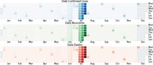
Figure 4.1 Cases in Karnataka, India.
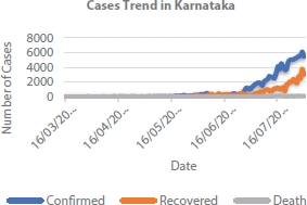
Figure 4.2 Cases trend in Karnataka, India.
4.2 Survey of Models
4.2.1 SEIR Model
SEIR model is a numerical model used to characterize the dynamics of epidemic outburst. This can be further used to predict the infection rate of growth based on metaheuristic method. Differential equations can be used to represent the variation of data based on infected, dead, recovered, quarantined, and protected using BFGS optimization algorithm [15].
4.2.2 Modified SEIR Model
The SEIR model which uses the time-series data is used to predict the contagion scenarios of the epidemic outbreak.
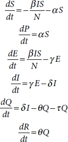
The interaction with six different parameters, namely, susceptible (S), exposed (E), infective (I), recovered (R), protected (P), quarantined (Q), and deaths (D) is shown in Figure 4.3.
SEIRPDQ model is described by a series of ordinary differential equations (4.1) [2]:
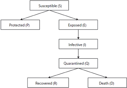
Figure 4.3 Modified SEIR.
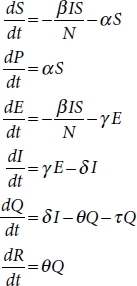
These equations depend on parameters β, α, γ, δ, θ, and τ [12].
β is infection rate.
α is the protection rate.
γ is the inverse of the average latent time
δ is the inverse of the average time
required to quarantine a person with symptoms.
θ is the recovery rate.
τ is the death rate.
Susceptible (S) is a group of individuals who are exposed to contagious people and possibility is high to get infected if they are in contact. If strict lockdown and social distancing regulations are followed, then the susceptible populations are protected (P). The infective population represents the infected people who have contacted with the contagious person. The quarantine (Q) group is that population who are quarantined in hospitals or home. They represent the actual cases detected that are able to pass the disease to susceptible people. Recovered (R) people get immunity so that they are not susceptible to the same illness anymore. Death indicates the deceased population [4, 5].
4.2.3 Long Short-Term Memory (LSTM)
To predict the growth of an epidemic, the information of the history of the events is required. It is difficult for a traditional neural network to predict the future based on the history. The class of neural network is known as RNN which will address the issue. These networks have a feedback path allowing the history of events to persist [6]. The RNNs has good performance in connecting the previous information to the present task. Traditional RNNs cannot connect the present task to the long running history of events due to an issue called vanishing the gradients. Here, the effect of past event will connect to the present gradient. This RNN connects the present task to its history with small number of events occurred [13].
To address the issue in the RNN, a class of RNN that works better than the traditional RNN in various fields such as natural language processing, stock market predictions, and sentiment prediction was considered. This model was used for the prediction of COVID-19 and the exact manifestation is still limited because availability of quality data. A LSTM model was designed to predict the cases in China by training the model over 2003 SARS data, and it was predicted that the cases will be hiked in February 2020 followed by gradual decrease [3]. By default, LSTMs are designed to learn the long-term dependencies. In general, all RNNs have chain like structure of repeating blocks/models of simple neural network [6]. The LSTM is able to learn term dependencies and remember the long-term values as per the requirement [7].
The basic structure of the LSTM is as shown in Figure 4.4. Each block/model has three main gates, namely, Forget gate (f), Update gate (i), and Output gate (o). The value of this gate ranges from 0 to 1. The gates decide the percentage of data to be remembered from the previous value which needs to be updated to the present value from the learned history.
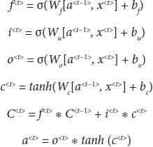
As shown in Figure 4.4, the LSTM cell will have three inputs in which two inputs are from the previous cell which will contribute to remember the history of events. These inputs are called as memory component C<t> and activation component a<t>. The third input is the tth time stamp x<t> of the data set X. The LSTM cell validates the inputs and updates the remembering and forgetting capacities which, in turn, produces the memory and the activation component for the next timestamp. The LSTM cell is a standard cell activation function and all the linear combinations are predefined by Equation (4.2) [7].
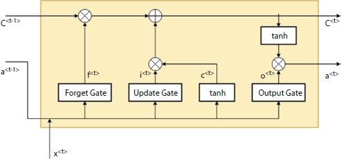
Figure 4.4 LSTM cell.
4.3 Methodology
The algorithm used for prediction of epidemic using both modified SEIR and LSTM model is discussed. SEIR methodology describes the deduction of a differential equation with the considered parameters. The change in the values of the parameters affects the response of the S, E, I, R, P, and Q values. For the parameter optimization, the curve with low value of RMSLE will predict the pandemic accurately. The time forecasting of the COVID-19 data is built and trained on a LSTM network using RMSLE loss function and Adam optimizer. The data pre-processing, algorithm, and the prediction are mentioned in the later section.
4.3.1 Modified SEIR
STEP 1: The parameters used in the equations are initialized. The parameters are as follows:
N: Total population
I: Infected (1)
R: Recovered (0)
E: Exposed (0)
S: N-I-R-E-P-Q
Beta: infectious rate (B)
Gama: 1/average latent time (G)
Lambda: recovery rate (L)
Kappa: death rate (K)
Alpha: protection rate (A)
Sigma: quarantine factor (S)
STEP 2: SEIRDP function is defined which returns the differential equations as indicated in Equation (4.3)
STEP 3: To solve the equations
Generally, to solve the linear differential equations, we can use Laplace transforms. Here, we use python SciPy. Integrate package using function ODEINT
Integrating equation using odient function: Solution = odient(model, y0,t)
- • Model is the SEIRDP function which contains all the model equation.
- • Initializing the differential states and time points are defined.
Integration and returning SEIRPQ values.
STEP 4: The differential equations and solutions should be trained to our model in order to fit the data curve with the actual curve. In total, 80% of data is used to train the model and 20% data is used to test the model [9].
STEP 5: Defining the opt_seir function and err_seir function which returns integration and root mean squared value respectively which are used to optimize the parameters.
Opt_seir function is used to optimize the parameters below which was previously initialized. Optimization is done using a function called BFGS the optimized parameter values are obtained
Beta: infectious rate (B)
Gama: 1/average latent time (G)
Lambda: recovery rate (L)
Kappa: death rate (K)
Alpha: protection rate (A)
Sigma: quarantine factor (S)
STEP 6: Optimization is done using a function called Broyden Fletcher Goldfarb Shanno (BFGS); the optimized parameter values are obtained:
Solution = odient(model,y0,t)
- • Model is the SEIRDP function which contains all the model equation.
- • Optimized parameter values are uploaded here.
- • Integration and returning SEIRPQ values.
4.3.2 LSTM Model
4.3.2.1 Data Pre-Processing
Data pre-processing is required to train any model to make sure that the training process behaves better by improving the numerical condition of the optimizer. This will also ensure that the various initializations are made appropriately [10]. LSTM networks are very sensitive to the scaling and the min max scaler works best for the LSTM network. This normalization will also help in removing unnecessary bias to the training and validation data [10]. The min max scaler equation is as shown in Equation (4.4):
where X is the data set and the Xscaled is the normalized data set.
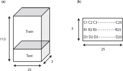
Figure 4.5 (a) Arrangement of data set in 3D tensor. (b) Mapping of the 3D and 2D tensors.
4.3.2.2 Data Shaping
The designed LSTM model takes input of 25days data (window = 25) and predicts the 26th day’s data. The cumulative number of confirmed, recovered, and death cases for each day and predict the number for the next day is compiled. In the proposed work, data of 138 days from 16th of March 2020 to 31st of July 2020 is used for training and testing of the model. The number of training to testing ratio is 80:20. Since we have window of 25, the total number of data set generated is 138 – 25 = 113. These data are arranged in 3D numpy array as shown in Figure 4.4 since the LSTM model demands the data to be in 3D tensor with shape (number of data set, time stamp, input features) = (113, 25, 3) [11]. This 3D array is divided into training and testing data, training data input shape = (90, 25, 3) and testing data input shape = (23, 25, 3), each of these data will have the label as the next day’s data; therefore the output will be (90, 3) and (23, 3), respectively.
The 3D tensor is as shown in Figure 4.5a. The ith row of the 3D tensor will have a 2D tensor as shown in Figure 4.5b, where Ck=25 denotes the confirmed cases, Rk=25 denotes recovered cases, and Dk=25 denotes the number of deaths.
4.3.2.3 Model Design
The deep learning model is designed with LSTM which takes 25 timestamped input to predict the number of cases for the next day. The model is designed with two hidden layers with each consisting of 45 hidden units. These hidden layers output is then connected to the output dense layer with three units. These three units are confirmed, recovered, and death cases, respectively. The summary of the model is as shown in Table 4.1[8].
Table 4.1 Model summary.
| Model: "sequential" | ||
| Layer (type) | Output shape | Param # |
| lstm (LSTM) | (None, 25, 45) | 8,820 |
| dropout (Dropout) | (None, 25, 45) | 0 |
| lstm_1 (LSTM) | (None, 45) | 16,380 |
| dropout_1 (Dropout) | (None, 45) | 0 |
| dense (Dense) | (None, 3) | 138 |
| Total Params: 25,338 Trainable params: 25,338 Non-Trainable params: 0 | ||
The model is regularized using L1_L2 kernel regularization; L2 bias reg-ularization and a dropout of 0.2 to reduce the overfitting of the model.
The model is trained with a batch size of 32 by using an Adam optimizer with performance measuring loss function of root mean square logarithmic error (RMSLE) function defined by Equation (4.5).
where N is the total number of predicts, P is the predicted value, and A is the actual value.
The reason for using RMSLE as a loss function over other functions is that in presence of outliers other function might explode but RMSLE does not, also RMSLE as a unique property of measuring the relative error. Also, it penalizes the underestimation of the actual value more severely than it does for the overestimation.
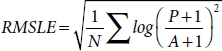
The significance of using loss function in the deep learning algorithm is to measure how well the algorithm is implemented in the model. For the model to train well, the error between the actual and the predicted values should be less. So, the process of training any model is to reduce this error. In the process the loss function fluctuates a lot which needs a suitable optimization. With the help of Adam optimizer, the RMSLE loss function will reduce the error in prediction and tries to smoothen the loss function curve. The loss function curve over the epoch is as shown in Figure 4.6.
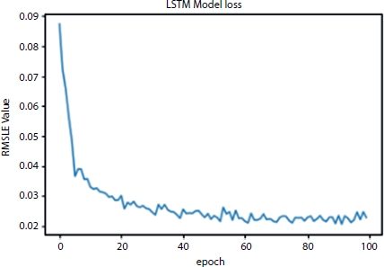
Figure 4.6 RMSLE value vs. number of epochs.
The model is then trained with the learning rate of 0.001. However, a reduce learning on plateau is used as a callback to vary the learning rate accordingly [14].
4.4 Experimental Results
4.4.1 Modified SEIR Model
The time series results are obtained by the standard deterministic approach for SEIR mode. Data is analyzed for Karnataka framework at a regional scale, and the results are computed. The interpretation of the Karnataka situation according to the deterministic solver shows the trends given in Figure 4.7. The plot indicates confirmed cases (infection), active cases, recovered, and death cases with respect to the number of days.
The sum of the active cases, recovered, and death cases gives the confirmed cases at that date. The model is trained with the given data by considering the following six parameters: infectious rate, recovery rate, death rate, protection rate, quarantine rate, and average latent time by using optimization function and curve fit function. For verifying the actual working of the model, 80% data is used for the training and 20% data is considered as testing data to minimize the error and fit the data. One hundred thirty-eight data samples are considered starting from March 16, 2020 to July 31, 2020. From this, 111-day data was used for training of our SEIR model. Test case data fitting in SEIR model is shown in Figure 4.8.
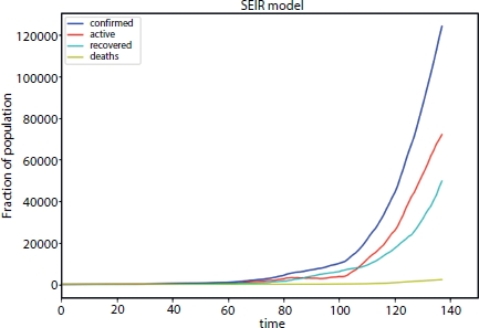
Figure 4.7 Cases in Karnataka.
Figure 4.8 SEIR Model fit for test cases.
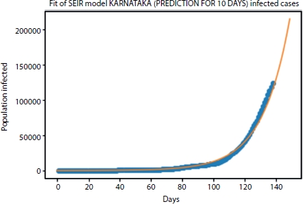
Figure 4.9 Cases predicted for next 10 days.
The orange and blue lines represent the fitted curve and actual curve, respectively. From Figure 4.7 the curve is approximately fitted with the RMSLE of 0.0304. If we increase the data training state and consider other factors such as medical facility available, medications, and hygiene factors in the mathematical modeling, then the exact curve fitting is achieved. In this context, six different parameters of infectious rate, recovery rate, death rate, protection rate, quarantine rate, and average latent time are considered to estimate the infection in the next 10 days using SEIR model that is as shown in Figure 4.9.
From the graph, we estimate that the cases after next 10 days will be around 18.8 lakhs.
4.4.2 LSTM Model
The LSTM is a neural network model which consists of the layers of neurons connected to each other and has associated parameters. These parameters are obtained through a better training of the model. The LSTM network could have captured the growth of the epidemic with better RMSLE when provided with the larger number of data (big data). The validation results obtained after training the LSTM model with the mentioned parameters are computed [16]. The graph plotted with actual and predicted number of cases for test data set is as shown in Figure 4.10. From Figure 4.10, the curve is approximately fitted with the RMSLE as 0.05438.
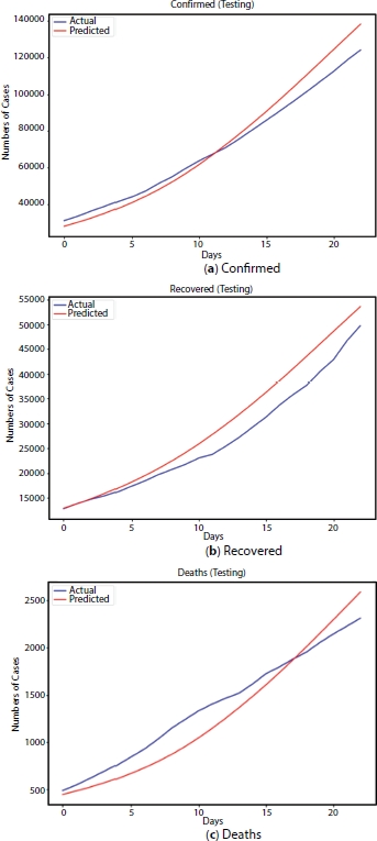
Figure 4.10 Testing results.
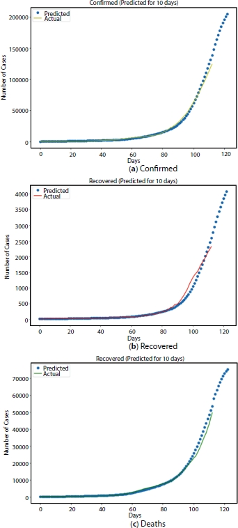
Figure 4.11 Next 10 days Prediction using LSTM model.
The prediction for subsequent 10 days is as shown in Figure 4.11. It is found that the confirmed cases after 10 days, i.e., on 11th of August 2020 may be around 2.12 lakh and recovered may be around 77,000 and there might be around 4,200.
4.5 Conclusion
The modified SEIR and LSTM model discussed in the paper is used to forecast the number of cumulative, recovered, and death cases in the state of Karnataka. In this context, the parameters considered are not time dependent leading to higher prediction error. The error in the SEIR will increase the values of parameters such as infectious rate, death rate, latent time, quarantine rate. The LSTM model implemented has RMSLE of 0.017 which implies less error in LSTM which leads to closer prediction toward the actual value.
Table 4.2 indicates the error in the LSTM model does not change much. The error in prediction from SEIR model varies linearly with increase in number of predictions days. This implies that the SEIR model cannot be used for the prediction of the epidemic data after a long period of time, whereas LSTM works effectively even for a longer duration when compared with the SEIR model. The variation of prediction error with respect to the number of days shown in Figures 4.12 and 4.13 implies that LSTM performs better than modified SEIR.
4.6 Future Work
The SEIR model can be further optimized such that the error does not increase with increase in number of days of predictions also the neural network model can be optimized and can also be tried on other networks and compare the performance of each network on same data. As the deep learning models are data hungry models and presently, the model has been tried on data of 138 days, which is not that sufficient to optimize the model. The model can be reworked with increased data and also be tried on other networks and optimizers and compare each of them.
Table 4.2 Predicted data.
| Date | Actual | Modified SEIR | ||
| Predicted | RMSLE | % Error | ||
| 01-08-2020 | 129287 | 120832 | 0.029372 | -6.54 |
| 02-08-2020 | 134819 | 127985 | 0.022591 | –5.07 |
| 03-08-2020 | 139571 | 135562 | 0.012657 | –2.87 |
| 04-08-2020 | 145830 | 143588 | 0.006728 | –1.54 |
| 05-08-2020 | 151449 | 152089 | 0.0018313 | 0.42 |
| 06-08-2020 | 158254 | 161093 | 0.0077219 | 1.79 |
| 07-08-2020 | 164924 | 170630 | 0.0147714 | 3.46 |
| 08-08-2020 | 172102 | 180731 | 0.0212466 | 5.01 |
| 09-08-2020 | 178087 | 191431 | 0.031379 | 7.49 |
| 10-08-2020 | 182354 | 202764 | 0.0460753 | 11.19 |
| 11-08-2020 | 188611 | 214768 | 0.0564022 | 13.87 |
| Date | Actual | LSTM | ||
| Predicted | RMSLE | % Error | ||
| 01-08-2020 | 129287 | 148020 | 0.0587651 | 14.49 |
| 02-08-2020 | 134819 | 155899 | 0.0630917 | 15.64 |
| 03-08-2020 | 139571 | 163532 | 0.0688071 | 17.17 |
| 04-08-2020 | 145830 | 170832 | 0.0687219 | 17.14 |
| 05-08-2020 | 151449 | 177725 | 0.0694816 | 17.35 |
| 06-08-2020 | 158254 | 184156 | 0.0658307 | 16.37 |
| 07-08-2020 | 164924 | 190088 | 0.0616704 | 15.26 |
| 08-08-2020 | 172102 | 195506 | 0.0553738 | 13.6 |
| 09-08-2020 | 178087 | 200410 | 0.0512868 | 12.53 |
| 10-08-2020 | 182354 | 208744 | 0.0586984 | 14.47 |
| 11-08-2020 | 188611 | 212229 | 0.0512374 | 12.52 |
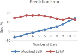
Figure 4.12 Prediction error curve.
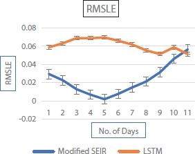
Figure 4.13 Prediction error and RMSLE curve.
References
1. Health and Family welfare Department, Government of Karnataka, Karnataka, 2020, COVID19 data: https://covid19.karnataka.gov.in/english.
2. COVID-19 dynamics with SIR model. Stochastic Epidemic Models with Inference, Springer 1st edition, 2019, https://www.lewuathe.com/covid-19-dynamics-with-sir-model.html.
3. Yang, Z., Zeng, Z., Wang, K., Wong, S.S., Liang, W., Zanin, M., Liu, P., Cao, X., Gao, Z., Mai, Z., Liang, J., Liu, X., Li, S., Li, Y., Ye, F., Guan, W., Yang, Y., Li, F., Luo, S., Xie, Y., Liu, B., Wang, Z., Zhang, S., Wang, Y., Zhong, N., He, J., Modified SEIR and AI prediction of the epidemics trend of COVID-19 in China under public health interventions. J. Thorac. Dis., 12, 3, 165–174, 2020.
4. Calafiore, G.C., Novara, C., Possieri, C., A Modified SIR Model for the COVID-19 Contagion in Italy. Computational Engineering,Finance, and M-SEIR & LSTM for Prediction of COVID-19 119 Science (cs.CE); Social and Information Networks (cs.SI); Systems and Control (eess.SY), arXiv:2003.14391, 31 Mar 2020.
5. Tiwari, A., Modelling and analysis of COVID-19 epidemic in India, J. Safety Sci. Resilience, 1, 2, 135–140, Dec 2020. medRxiv 2020.04.12.20062794; https://doi.org/10.1101/2020.04.12.20062794.
6. OlahLSTM-NEURAL-NETWORK-TUTORIAL-15. Understanding LSTM Networks, 27 August 2015, https://web.stanford.edu/class/cs379c/archive/2018/class_messages_listing/content/Artificial_Neural_Network_Technology_Tutorials/OlahLSTM-NEURAL-NETWORK-TUTORIAL-15.pdf
7. Yudistira, N., COVID-19 growth prediction using multivariate long short-term memory, J. Latex Class Files, 14, 8, August 2015, arXiv: 2005.04809v2.
8. Sujath, R., Chatterjee, J.M., Hassanien, A.E., A machine learning forecasting model for COVID-19 pandemic in India. Stoch. Environ. Res. Risk Assess., 34, 959–972, 2020, https://doi.org/10.1007/s00477-020-01827-8.
9. Mollalo, A., Rivera, K.M., Vahedi, B., Artificial Neural Network Modeling of Novel Coronavirus (COVID-19) Incidence Rates across the Continental United States,. Int. J. Environ. Res. Public Health, 17, 12, June 2020.
10. ftp://ftp.sas.com/pub/neural/FAQ2.html 11 October 2002.
11. Verma, S., Understanding Input and Outputshape in LSTM (Keras). Towards Data Science,2019, https://mc.ai/understanding-input-and-output-shape-in-lstm-keras/.
12. SEIR Modeling of the Italian Epidemic of SARS-CoV-2 Using Computational Swarm Intelligence. Int. J. Environ. Res. Public Health, 17, 10, May 2020.
13. https://github.com/anasselhoud/CoVid-19-RNN
14. MATLAB code for SEIR model. Mathworks, 2020, https://in.mathworks.com/matlabcentral/fileexchange/74545-generalized-seir-epidemic-model-fitting-and-computation.
15. Karnataka COVID19 timeline, https://en.wikipedia.org/wiki/COVID-19_pandemic_in_Karnataka, Wikipedia, 2020.
16. https://github.com/Aveek-Saha/CovidAnalysis/blob/master/LSTM_modeling.ipynb
- *Corresponding author: [email protected]