
3
Model Evaluation
Ravi Shekhar Tiwari
University of New South Wales, Kensington, Sydney, Australia
Abstract
We are in a technology-driven era, where 70% of our activities are directly dependent on technology and the remaining 30% is indirectly dependent. During the recent time, there was a breakthrough in computing power and in the storage devices—which gave rise to technology such as cloud, Gpu, and Tpu—as a result of our storage and processing capacity increased exponentially. The exponential increase in storage and computing capabilities enables the researcher to deploy Artificial Intelligence (A.I.) in a real-world application.
A.I. in real-world application refers to the deployment of the trained Machine Learning (ML) and Deep Learning (DL) models, to minimize the human intervention in the process and make the machine self-reliant. As we all know, for every action, there is a positive and negative reaction. These breakthroughs in the technology lead to the creation of a variety of ML/DL models but the researchers were stupefied between the selection of models. They were bewildered which model they should select as to correctly mimic the human mind—the goal of A.I. As most of us are solely dependent on the accuracy metric to justify the performance of our model, but in some cases, the accuracy of the simple model and complex model are almost equivalent. To solve this perplexity, researchers came up with a variety of the metrics which are dependent on the dataset on which the ML/DL model was trained and on the applications of the ML/DL models. So, that individual can justify their model—with the accuracy metric and the metrics which are dependent on the dataset as well as the application of the respective model. In this chapter, we are going to discuss various metrics which will help us to evaluate and justify the model.
Keywords: Model evaluation, metrics, machine learning models, deep learning models, Artificial Intelligence
3.1 Introduction
We are expected to enter in the era of Machine General Intelligence, which allows machine to have intelligence to perform most of the human work technically but its foundation lies on the various techniques of the Machine Learning (ML) and one of the most important part of ML is evaluation of model. In recent days, we are aware of the scenario where more than one model exists for our goal or objective. Some of the models are complex—lacks explain ability where as some of them are simple and can be explained. Recent development in the Artificial Intelligence (A.I.) has given us the capacity to explain the prediction of the models using Shapley, LIME, and various ML explain ability tools, but still we are in dilemma when it comes to choose the best model for our objective.
“Swords cannot be replaced Needle”—although it has unlimited power when compared to needle. Similarly, it is better to choose simple model with respect to the complex model when there is minute difference in the accuracy because it will be computational economical when compared to complex model which uses far more resources. But in some use cases, we cannot rely totally on the accuracy—it is just the quantitative value of correct prediction from model with respect to the total number of samples. Accuracy can prove inefficient as well as incorrect quantitative value when it comes to imbalance dataset. Imbalance dataset is the term use to denote the dataset when sample from the classes is not equal; in this case, accuracy is not in a position to justify our model.
Model evaluation is one of the core topics in ML which help us to optimize the model by altering its parameter during training phase. Though accuracy is one of the pillars of model evaluation, it is reinforced with over supporting evaluation metric to justly the usefulness of the model. In this chapter, we are going to learn metrics some of them acts as a pillar for the ML models, and some of them acts as a supporting metrics. The chapter is basically categorized into four parts: regression, correlation, confusion metric, and natural language processing metric with pseudo code, which brings the clarity about the metrics, and their uses, as well as pros and cons, respectively.
3.2 Model Evaluation
Model evaluation is one of the most crucial processes after training and testing the model because we have restriction of computation as well as on the bandwidth of data which will serve as an input to these trained models; hence, it is not feasible to deploy complex model whose accuracy is almost equivalent to simple model because most of the time accuracy metric is not enough to justify our model (in case of imbalance class) [1]. We need to justify our model productivity by comparing it with another trained model or base model, so we need different types of metrics such as R2, adjusted R2, and RMSE, to describe the trend of data concerning the regression line, error, as well as other statistical quantitative metrics [7].
Figure 3.1 is a brief representation of the process or the procedures which take place before the deployment of any ML/DL model.
Regression is defined as the statistical term which attempts to determine the relationship between the independent variable (IV) which will be denoted by X and dependent variable (DV) which will be denoted by Y [3]. In the regression model, we train the model on IV, i.e., X, and try to predict DV, i.e.,Y, where the value of X and Y ranges from [–infinity, + infinity]. Classification refers to the process of categorizing or assigning the input data in one of the classes.
Let us first make some assumptions and understand some terminologies which will help to understand the coming evaluation metrics easily.
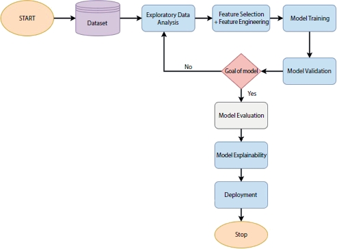
Figure 3.1 ML/DL model deployment process.
3.2.1 Assumptions
Suppose you build a regression model whose equation is Y = mx + c + ε, where m is the slope of line, c is the intercept, ε is the error, and x is the input variable [6]; in the case of linear regression, m and c refer to weight and bias, which are learned by the model oven e epochs on n samples. The predicted value from the model is O and the actual value is Y.
3.2.2 Residual
It is defined as the difference between actual value Y{i} and predicted value O{i}. Refer to Figure 3.2 where dots represent the actual value Y and the value predicted value O by our model. Since our model is the regression model, I have shown it with line denoted by Y = mx + c, whose output will be a point on the line Y which is dependent on x. It is also known as residual [3].
If we substitute the value of Y = mx{i} + c + ε and O = mx{i} + c in Equation (3.1), we will get
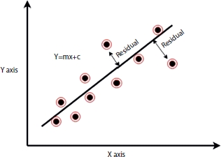
Figure 3.2 Residual.
3.2.3 Error Sum of Squares (Sse)
It quantifies how much the data points Y{i} is far from points on the regression line, i.e., Y{i} = mx{i} + c + ε, varies around the estimated regression line, i.e., and O{i} = mx{i} + c [4].
If we substitute the value of Y = mx{i} + c + ε and O = mx{i} + c in Equation (3.3), then we will get
3.2.4 Regression Sum of Squares (Ssr)
It quantifies how much the predicted output “O” estimated from the line O{i} = mx{i} + c is far from the “no relationship line”, i.e., ![]() .
.
If we substitute the value of ![]() and O = mx{i} + c in Equation (3.5), then we will get
and O = mx{i} + c in Equation (3.5), then we will get
3.2.5 Total Sum of Squares (Ssto)
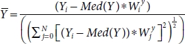
It is defined as the sum of Ssr and Sse, which quantifies, by how much data point from regression line, i.e., Y{i} = mx{i} + c + ε vary around their mean, i.e., ![]() [4].
[4].
If we substitute the value from Sse [Equation (3.3)] and Ssr [Equation (3.6)] in Equation (3.7), then we will get
By solving this equating using Equation (3.8), then we will get
3.3 Metric Used in Regression Model
As we say, the building is as strong as its foundation, we have built our foundation, and it is quite strong. So, we can start building floors one by one; hence, we will start with metrics which are extensively used in the regression model.
3.3.1 Mean Absolute Error (Mae)
Mae stands for Mean Absolute Error. Mae used to calculate overall mean variation between the prediction O from the estimated line O = mx{i} + c and actual value Y line Y = mx{i} + c + ε [6]. If we try to traverse from right to left, then we can split the terms into three individual terms: Error, Absolute, and Mean, respectively. These three words are related to each other in order of their split-up.
Error: It is also known as residuals (Figure 3.2), defined as the difference in the predicted value O and the actual value Y
Absolute: The error or residual of the model can have positive as well as a negative value. If we consider the negative value along with the positive value, then there are chances that positive and negative residuals of the same magnitude can negate each other which can have an adverse effect while backpropagation. Suppose our model has residuals of 2, 4, 6, 7, and –2, and if we take the mean of the error then value with the same magnitude, but the opposite sign can cancel each other, hence it will have an adverse effect on the model. So, by considering only the strength or magnitude of the error by taking absolute value, i.e., modulus of error, it is highly affected by the outlier [7].
If we substitute the value of Equation (3.10) in Equation (3.11), then we will get
Mean: We repeat the above steps, i.e., Error and Absolute for n-samples, i.e., the number of samples of which model is trained or tested and calculate mean and select the model which has minimum Mean Absolute Error.
If we substitute the value of Equation (3.12) in Equation (3.13), then we will get

The pseudo-code is given below for Mse:
For I in no. _samples:
Error = Y{i} – O{i}
Absolute = | Error |
Total Error = Total Error + Absolute
Mae = Total Error / no._samples
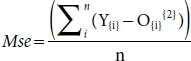
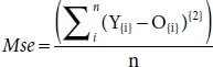
3.3.2 Mean Square Error (Mse)
Mse stands for Mean Square Error. Mae used to calculate overall mean square of variation between the prediction O from the estimated line O = mx{i} + c and actual value Y estimated line Y = mx{i} + c + ε [8]. If we try to traverse from right to left, we can split the term into three individual terms Error, Square, and Mean, respectively. These three words are related to each other in order of their split-up.
Error: It is also known as residuals (Figure 3.2), defined as the difference in the predicted value O and the actual value Y.
Square: The error or residual of the model can have positive as well as a negative value. If we consider the negative value along with the positive value, then there are chances that positive and negative residuals of the same magnitude can negate each other which can have an adverse effect while backpropagation. Suppose our model has residuals of 2, 4, 6, 7, and –2, and if we take the mean of the error then value with the same magnitude, but the opposite sign can cancel each other, hence it will have an adverse effect on the model. So, we square the error to handle the above-mentioned issue, whereas in Mae, we use the modulus operator [8].
If we substitute the value of Equation (3.15) in Equation (3.16), then we will get
Mean: We repeat the above steps, i.e., Error and Square for n-samples, i.e., the number of samples of which model is trained or tested and calculate mean and select the model which has minimum Mean Square Error.
If we substitute the value of Equation (3.17) in Equation (3.18), then we will get
The pseudo code is given below for Mse:
For I in no. _samples:
Square = (Error){2}
Total Error = Total Error + Square
Mse = Total Error / no._samples
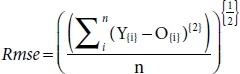
3.3.3 Root Mean Square Error (Rmse)
Rmse stands for Root Mean Square Error. Rmse used to calculate the overall root of the mean square of the variation between the prediction O from the estimated line O = mx{i} + c, and actual value Y line Y = mx{i} + c + ε. It is derived from the mean square error and is highly affected by the presence of outliers [10]. In RMSE, root empowers to show a large number of deviations, and when compared to Mae, it gives high weights to error and hence punishes the large errors [12]. If we try to traverse from right to left, then we can split the term into four individual terms: Error, Square, Mean, and Root, respectively. These four words are related to each other in order of their split-up.
Error: It is also known as residuals (Figure 3.2), defined as the difference in the predicted value O and the actual value Y.
Square: The error or residual of the model can have positive as well as a negative value. If we consider the negative value along with the positive value, then there are chances that positive and negative residuals of the same magnitude can negate each other which can have an adverse effect while backpropagation. Suppose our model has residuals of 2, 4, 6, 7, and –2, and if we take the mean of the error then value with the same magnitude, but the opposite sign can cancel each other, hence it will have an adverse effect on the model [10].
If we substitute the value of Equation (3.20) in Equation (3.21), then we will get
Mean: We repeat the above steps, i.e., Error and Square for n-samples, i.e., number of samples of which model is trained or tested and calculate mean. It is highly affected by outliers [11].
If we substitute the value of Equation (3.22) in Equation (3.23), then we will get
Root: After calculating the mean of the square of the error, we raise it to power ½, i.e., we take second root of Mse, hence ![]() . Second root gives high weight to the error, and as a result, it punishes large errors. We select the model which has minimum Mean Square Error.
. Second root gives high weight to the error, and as a result, it punishes large errors. We select the model which has minimum Mean Square Error.
If we substitute the value of Equation (3.24) in Equation (3.25), then we will get
The pseudo-code below for Rmse:
For I in no._samples:
Error = Y{i} – O{i}
Square = (Error){2}
Total Error = Total Error + Square
Mse = Total Error / no._samples
Rmse = (Mse)
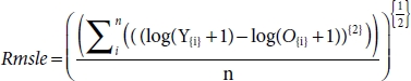
3.3.4 Root Mean Square Logarithm Error (Rmsle)
Rmsle stands for Mean Square Logarithm Error. Rmsle used to calculate the root of mean logarithm square of the variation between the prediction O from the estimated line O = mx{i} + c, and actual value Y line Y = mx{i} + c + ε. It is derived from the root mean square error and used when we do not want to penalize the huge error [16]. If we try to traverse from right to left, then we can split the term into five individual terms: Error, Logarithm, Square, Mean, and Root, respectively. These five words are related to each other in order of their split-up.
Logarithm: In this, we take the logarithm of the target value Y{i} and the predicted value O{i} and then we calculate the error. We all add 1 to these values to avoid taking the log of 0 [11, 16].
Error: It is also known as residuals (Figure 3.2), defined as the difference in the predicted value O and the actual value Y, but in Rmsle calculate error by taking the log of target and predicted value.
If we substitute the value of Equation (3.27) and of Equation (3.28) in Equation (3.29), then we will get
Square: The error or residual of the model can have positive as well as a negative value. If we consider the negative value along with the positive value, then there are chances that positive and negative residuals of the same magnitude can negate each other which can have an adverse effect while backpropagation. Suppose our model has residuals of 2, 4, 6, 7, and –2, and if we take the mean of the error then value with the same magnitude, but the opposite sign can cancel each other, hence it will have an adverse effect on the model.
If we substitute the value of Equation (3.30) in Equation (3.31), then we will get
Mean: We repeat the above steps, i.e., Error and Square for n-samples, i.e., number of samples of which model is trained or tested and calculate mean.
If we substitute the value of Equation (3.32) in Equation (3.33), then we will get msle (mean square log of error)

Root: After calculating the mean of the square of the error, we raise it to power ½, i.e., we take second root of Msle, ![]() . Second root gives high weight to the error, and as a result, it punishes large errors. We select the model which has minimum Mean Square Error.
. Second root gives high weight to the error, and as a result, it punishes large errors. We select the model which has minimum Mean Square Error.
If we substitute the value of Equation (3.34) in Equation (3.35), then we will get
The pseudo-code is given below for Rmsle:
For I in no._samples:
Logarithm of target = log (Y{i} + 1)
Logarithm of prediction = log (O{i} + 1)
Error = Logarithm of target – Logarithm of prediction
Square = ( Error){2}
Total Error = Total Error + Square
Msle = Total Error / no._samples
Rmsle (Msle)
If value O and Y values are small, then RMSE is equal to RMSLE, i.e., RMSE == RMSLE.
If any one of O and Y values are big, then RMSE is greater than RMSLE, i.e., RMSE > RMSLE.
If value O and Y values are big, then RMSE is very greater RMSLE, i.e., RMSE >> RMSLE.
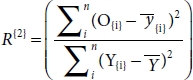
3.3.5 R-Square (R2)
R2 is also known as the coefficient of determination and is used to determine the goodness of fit, i.e., how well the model fits the line or how data fit the regression model [31]. It determines the proportion of variance in the DV that can be explained by IV. It ranges between [0, 1], where the model whose R2 value is close to 1 is considered a good model, but in some cases, this thumb rule also fails to validate [17]. It can be calculated by squaring the correlation between predicted and the actual value [30]. So, we need to consider the other factors also along with the R2 [18]. In simple words, we can say how good is our model when compared to the model which just predicts the mean value of the target from the test set as predictions [12].
where Sse is Error Sum of the square from Equation (3.38) and Ssto is Total Sum of the square from Equation (3.39), and replacing the values, respectively, then we get
By solving expanding Equation (3.37) using Equations (3.38), (3.39), and (3.40), we will get
So, Equation (3.42) can also be defined as
In simple words, we can say how good is our model when compared to the model which just predicts the mean value of the target from the test set as predictions.
3.3.5.1 Problem With R-Square (R2)
As I have mentioned above, R2 determines the proportion of variance in the DV that can be explained by IV and in Equation (3.43) to maximize the R2, we need to maximize MSE (model) or decrease MSE (baseline model) which predicts mean of the target variable. So, when we increase the IV and estimated equation change from Y = mx{i} + c + ε to Y = mx{i} + c + ε. Now, if the IV is not significantly correlated, then MSE (Baseline model) should increase and MSE (model) should decrease as a result of Equation (3.43), R2, the value should decrease but it was found that in reality the value of R2 does not decrease it keeps increasing [12]. As a result, adjusted R2 came to existence which is an improvised version of R2.
3.3.6 Adjusted R-Square (R2)
We have already discussed the problem related to R-square (R2), which is biased, i.e., R2 is biased—if we add new features or IV, then it does not penalize the model respective of the correlation of the IV. It always increases or remains the same, i.e., no penalization for uncorrelated IV [12]. To counter this problem, penalizing factor has been introduced in the Equation (3.41), which penalize R2.
where k = number of features and n = number of samples in the training set.
Now, from Equation (3.44), if we add more features the denominator, i.e., (n – (k + 1)) should decrease, so the whole Equation (3.44) should increase. We have R2 in the equation and if R2 does not increases (1 – R{2}) term will be close to 1. Overall, we are deducting larger value from 1, hence AdjustedR{2} will be close to 0. So, we can summarize that the added IV does not have a significant correlation with the DV hence does not add any value of the model.
Since, we have a basic idea of AdjustedR{2} from the above paragraph and we can proceed |Y{i} – O{i}| forward with mathematical intuition. Our aim is to make the LHS of the Equation (3.44) close to 1. So, we need to minimize the term which can be split into two parts, i.e.,
For the Equation (3.44a), to be minimum, we need R2 to be maximum, hence the bigger number will be subtracted from 1 which will result in a smaller term.
For Equation (3.44b), by adding an independent term in the denominator, the value of the denominator will increase; hence, overall value of the equation will be minimum. Overall, if we analyze by considering both Equations (3.44a) and (3.44b), then we are mainly dependent on (3.44a) to be minimum (when R2 is greater), i.e., by adding an IV R2 increases, then the IV is adding value to the model; else, it does not add any value to the model.
3.3.7 Variance
Variance is defined as how far point/points of points from the mean of the data points are. It is used in decision trees as well as random forest and ensemble algorithms to decide the split of the node which has a continuous sample [12, 24]. It is inversely proportional to the homogeneity, i.e., more variance in the node less the homogeneity. It is highly affected by the outliers.
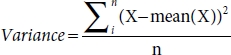
where X= data point, mean(X) = mean of all data point, and n = number of samples.
3.3.8 AIC
AIC refers to Akaike’s Information Criteria that is a method for scoring and selecting a model by considering Sse, number of parameter, and number of samples, developed by Hirotugu Akaik. AIC shows the relationship between Kullback-Leibler measurement and the likelihood estimation of the model [24]. It penalizes the complex model less, i.e., it emphasizes more on the training dataset by penalizing the model with an increase in the IV. AIC selects the complex model; the lower the value of AIC, better the model [24].
where N = number of parameters, LL = Log of Likelihood, and N = Number of samples
Here, in Equation (3.46), LL refers to the Log of Likelihood of the model for regression models; we can take LL as Mse and Ssr, and for classification, we can take Binary Cross Entropy. If we analyze Equation (3.46a), the term 2 ∗ k/N will be always positive since N and k are positive so this term will be greater than or equal to zero; also, in Equation (3.46b), the term –2/N ∗ LL will be negative always; the whole equation is a dependent parameter of the model instead of the number of samples, i.e., bigger the value of k, minimum the value of AIC.
3.3.9 BIC
BIC is a variant of AIC known as Bayesian Information Criterion [32]. Unlike the BIC, it penalizes the model for its complexity and hence selects the simple model [24]. The complexity of the model increases, BIC increases hence the chance of the selection decreases [24, 32]. BIC selects the simple model; the lower the value of BIC, the better the mode.
where N = number of parameters, LL = Log of Likelihood, and N = Number of samples
Here, in Equation (3.47), LL refers to the Log of Likelihood of the model for regression models; we can take LL as Mse and Ssr, and for classification, we can take Binary Cross Entropy. If we analyze Equation (3.47a), the term log(N) ∗ k will be always positive since N and k are positive so this term will be greater than or equal to zero; also, in Equation (3.47b), the term –2 ∗ LL will be negative always, and the whole equation is dependent on the number of samples of the training data of model, i.e., N increases, Equation (3.47b) increases, hence the value of Equation (3.47) decreases.
3.3.10 ACP, Press, and R2-Predicted
ACP is defined as Amemiya’s Prediction Criterion. The lower the value, the better the model.
where N = number of parameters, LL = Log of Likelihood, and N = Number of samples.
Press is a model approval technique used to evaluate a model’s prescient capacity that can likewise be utilized to look at relapse models [54]. For an informational collection of size n, Press is determined by precluding every perception exclusively, and afterward, the rest of the n – 1 perception is utilized to ascertain a relapse condition which is utilized to foresee the estimation of the discarded reaction esteem (which, in review, we indicate by O{ii}. We point that the ith Press remaining as the distinction Y{i} – O{ii}.
More modest the Press values, the better the model’s predicting capacity [54]. Press can likewise be utilized to compute the anticipated R2 (indicated by ![]() which is commonly more instinctive to decipher than Press itself. It is characterized as follows:
which is commonly more instinctive to decipher than Press itself. It is characterized as follows:
What is more, it is a useful method to estimate the prediction capacity of your model without choosing another example or parting the information into preparing and approval sets to evaluate the prediction of trained models. Together, Press and ![]() can help forestall overfitting because both are determined utilizing predictions excluded from the model assessment [54]. Overfitting alludes to models that seem to give a solid match to the informational index within reach, however, neglect to give substantial expectations to novel predictions. You may see that and R2 are comparative in structure [31, 54]. While they would not be equivalent to one another, it is conceivable to have R2 very high comparative with
can help forestall overfitting because both are determined utilizing predictions excluded from the model assessment [54]. Overfitting alludes to models that seem to give a solid match to the informational index within reach, however, neglect to give substantial expectations to novel predictions. You may see that and R2 are comparative in structure [31, 54]. While they would not be equivalent to one another, it is conceivable to have R2 very high comparative with ![]() , which suggests that the fitted model is overfitting the example information. Be that as it may, dissimilar to R2,
, which suggests that the fitted model is overfitting the example information. Be that as it may, dissimilar to R2, ![]() < 0 happens when the fundamental PRESS gets expanded past the degree of the SSTO. In such a case, we can just shorten
< 0 happens when the fundamental PRESS gets expanded past the degree of the SSTO. In such a case, we can just shorten ![]() at 0. At long last, if the PRESS value gives off an impression of being enormous because of a couple of exceptions, at that point, a minor departure from Press (utilizing the supreme incentive as a proportion of separation) may likewise be determined [54].
at 0. At long last, if the PRESS value gives off an impression of being enormous because of a couple of exceptions, at that point, a minor departure from Press (utilizing the supreme incentive as a proportion of separation) may likewise be determined [54].
3.3.11 Solved Examples
As we have understood several metrics, it will be better if we do one example from the above metrics. Let us assume that the predicted value is O = [2, 9, 4, 7, 8, 4, 1] and actual value, i.e., target value, is Y = [2, 6, 3, 5, 7, 8, 3], and the number of samples is 7, i.e., n(O) = n(Y) = 7 and number of parameters be 3.
By solving according to the formula of the metric, we will get the value which is mentioned in Table 3.1, and by using the above-mentioned formulas, we will get
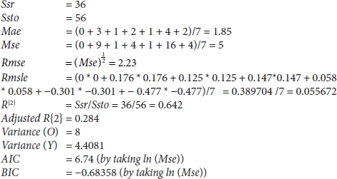
Table 3.1 Calculation and derived value from the predicted and actual values.
| Y | O | Y – O | |Y – O| | (Y – O)^2 | Log(Y + 1) | Log(O + 1) | Log(Y + 1) – Log(0 + 1) |
| 2 | 2 | 0 | 0 | 0 | 0.301 | 0.301 | 0 |
| 9 | 6 | 3 | 3 | 9 | 0.954 | 0.778 | 0.176 |
| 4 | 3 | 1 | 1 | 1 | 0.602 | 0.477 | 0.125 |
| 7 | 5 | 2 | 2 | 4 | 0.845 | 0.698 | 0.147 |
| 8 | 7 | 1 | 1 | 1 | 0.903 | 0.845 | 0.058 |
| 4 | 8 | –4 | 4 | 16 | 0.602 | 0.903 | –0.301 |
| 1 | 3 | –2 | 2 | 4 | 0 | 0.477 | –0.477 |
3.4 Confusion Metrics
Confusion metric is one of the most widely used metrics for classification [27]. From the confusion metric, several metrics can be derived which can be used to evaluate binary class classification models as well as multi-class classification such as TPR, accuracy, precision, and many others, which we are going to discuss. It applies to ML as well as DL models—the task is to predict labels of the input data into specific classes like dog or cat, bus, or car, which are encoded numerically [34].
Confusion metric is a metric of size m * m (m is no. of classes); if we traverse row-wise, i.e., left to right, then it represents Predicted Value, i.e., number of samples which were predicted correctly as well as predicted incorrectly [32, 34]. Similarly, if we traverse column-wise only, then it represents Actual Value, and the combination of the row and column gives the magnitude of the True Positive (TP), True Negative (TN), False Positive (FP), and False Negative (FN).
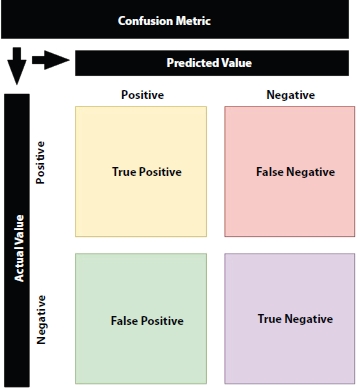
Figure 3.3 Confusion metric.
3.4.1 How to Interpret the Confusion Metric?
From Figure 3.3, we can split the confusion metric into four separate elements, i.e., TP, TN, FP, and FN [40]. As I have mentioned earlier and it is clear from Figure 3.3, the column represents Predicted Value, and the row represents the Actual Value. We all know that we read the elements of the metric by Row and then column. So, we will use True (T) and False (F) to denote the value column, i.e., actual value, and we will use Positive (P) and Negative (T) to denote the value row, i.e., predicted value.
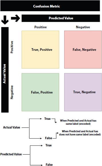
Figure 3.4 Confusion metric interpretation.
If we analyze from the Figure 3.4, we will see if the model predicts the label as Negative and in actual the value is Negative so we will call it as TN, True—since predicted and the actual value is same, and Negative—because model predicted the label as negative. Similarly, if the model predicts the label as Positive, and in reality, the value is Negative, so we will call it as FP, False—since predicted and the actual value is not the same, and Positive— because the model predicted the label as Positive.
From the confusion metric, we can derive the following data, which can be used to derive other metrics which will support the accuracy metric [55, 57].
FN = Prediction from the model is negative and the actual value is positive, so the trained model prediction is incorrect and known as FN—Type 2 error [56].
FP = Prediction from the model is positive and the actual value is negative, so the trained model prediction is incorrect and known as FP—Type 1 error [56].
TN = Prediction from the model matches the actual value, i.e., the model predicted the negative value, and the actual value is also negatively known as TN [56].

Figure 3.5 Metric derived from confusion metric.
TP = Prediction from the model matches the actual value, i.e., the model predicted the positive value, and the actual value is positively known as TP [56].
Confusion metric elements can be used to derive other metrics because the model which we train is dependent on the use case. These use cases sometimes vary where we want to prioritize accuracy or TPs or FPs. So, we need to justify the accuracy with other supporting metrics because in some cases accuracy fails to justify our model [1, 6]. Figure 3.5 shows the list of the metrics derived from the confusion metric.
Here, we will discuss each of the metrics mentioned in Figure 3.5 in detail.
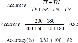
3.4.2 Accuracy
Accuracy is defined as the ratio of the total number of correctly predicted samples by the model to the total number of samples [55].
If we substitute the value of Equations (3.54) and (3.55) in Equation (3.56), then we will get
So,
3.4.2.1 Why Do We Need the Other Metric Along With Accuracy?
Suppose we have a dataset which has 90 dog images and 10 cat images, and a model is trained to predict dog, where a trained model predicted 80 correct samples and 20 incorrect samples.
So, in this case, if we calculate accuracy from Equation (3.52), then we will get the following:
From confusion metric, we can say,
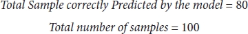
So,

Accuracy is quite good, so we can select the model!
No, because the dataset is imbalanced, and hence, we cannot depend totally on accuracy because 80% of the tie model is predicting—the image is not the cat. So, it is biased toward one class. So, we need supporting metrics to justify our model [6, 7].
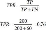
3.4.3 True Positive Rate (TPR)
TPR is known as True Positive rate, which is the ratio of TP: (TP + FN) or, in simple words, ratio of correctly predicted positive labels to the total actual positive labels [24, 31]. The value of TPR is directly proportional to the goodness of model, i.e., TPR increases, model becomes better and hence can be used as an alternative to the accuracy metric.
If we substitute Equations (3.58) and (3.59) in Equation (3.60), then we will get
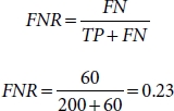
3.4.4 False Negative Rate (FNR)
FNR is known as False Negative rate, which is the ratio of FN: (TP + FN) or, in simple words, ratio of incorrect predicted positive labels to the total actual positive labels [24, 31]. The value of FNR is inversely proportional to the goodness of model, i.e., FNR decreases, model becomes better and hence can be used as an alternative to the accuracy metric.
If we substitute Equations (3.62) and (3.63) in Equation (3.64), then we will get
3.4.5 True Negative Rate (TNR)
TNR is known as True Negative rate, which is ratio of TN: (FP + TN) or, in simple words, ratio of correct predicted negative labels to the total actual negative labels [24, 31]. The value of TNR is directly proportional to the goodness of model, i.e., FPR increases, model becomes better and hence can be used as an alternative to the accuracy metric.
If we substitute Equations (3.66) and (3.67) in Equation (3.68), then we will get
3.4.6 False Positive Rate (FPR)
FPR is known as False Positive rate, which is ratio of FP: (FP + TN) or, in simple words, ratio of incorrect predicted negative labels to the total actual negative labels [24, 31]. The value of FNR is indirectly proportional to the goodness of model, i.e., FPR decreases, model becomes better and hence can be used as an alternative to the accuracy metric.
If we substitute Equations (3.70) and (3.71) in Equation (3.72), then we will get
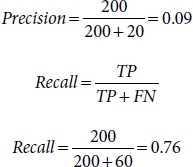
3.4.7 Precision
Precision tells us how many of the positive samples were predicted correctly to all positive predicted samples, i.e., TP: (TP + FP). We cannot afford to have more FP because it will degrade our model [22, 28].
If we substitute Equations (3.74) and (3.75) in Equation (3.76), then we will get
Suppose classification model is trained to identify the patients who will be vulnerable to death by Covid-19 by considering various features like age, lungs condition, medical history, and various explicit as well as implicit factors, it categorizes patient in two classes, i.e., class 0—low chance of death and class 1—high chance of death. In this, we cannot allow the model to give us the high value of FP, i.e., Type 1 error—the person is at high risk and the model is predicting the person is at low risk. Hence, we try to minimize the FP and maximize TP. This metric is used extensively in healthcare applications [34].
3.4.8 Recall
Recall tells us how many of the samples were predicted correctly to all the actual positive samples, i.e., TP : (TP + FN). We cannot afford to have more FN because it will degrade our model [22].
Suppose the classification model is trained to identify the persons who are criminal and have a high chance of indulging in illegal activities. In this case, our priority will be to reduce FN, i.e., Type 1 error. If FN is high, then there is an increased chance that a person who can indulge in illegal activities can escape and the innocent person can be put behind bars; hence, it will increase the crime rate in our society. Hence, we try to minimize the FN and maximize TP [35].
3.4.9 Recall-Precision Trade-Off
Recall considers actual positive label, whereas precision considers total predicted positive labels as their denominator, respectively [24, 25, 34].
So, they are inverse of each other where if one increases another decreases and vice versa. Hence, we have to choose among these two metrics according to the application of the trained ML/DL model.
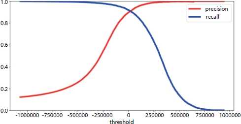
Figure 3.6 Precision-recall trade-off.
As shown in Figure 3.6, if we plot precision and recall, they intersect each other at a point where Precision == Recall [34]; this is known as precision-recall trade-off because if we move leftward or rightward from the intersection of these two lines, one value will decrease, and another will increase [24].
3.4.10 F1-Score
As we have discussed above that precision and recall are inversely related and, in some cases, where we are unable to decide between precision and recall, we proceed with F1-score which is the combination of precision and recall [43]. Precision is the harmonic mean of precision and recall has a maximum value when precision and recall are equal, i.e., they intersect each other. It is always used with other evaluation metrics because it lacks interpretation.
By solving Equation (3.86), then we will get
3.4.11 F-Beta Sore
We have discussed earlier that F-score uses geometric mean instead of the arithmetic mean because Harmonic mean punishes penalize bigger value more when compared to the arithmetic mean [43].
Consider a case where Precision = 0 and Recall = 1, then
By substituting the value of Precision and Recall in Equation (3.88), then we will get
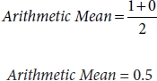
And if we take harmonic mean, i.e., F1-score, then we will get
If we analyze these two values, i.e., arithmetic mean and harmonic mean (F1-Score), and if we analyze the output of any random model that is equal to the arithmetic mean, hence F1-score (harmonic mean) penalizes the bigger value more as compared to the arithmetic mean.
F-beta score is the improvised version of the F1-score where the individual can give desired weight to the precision or recall [22, 43] according to the business case, or as per the requirement, the weight is known as beta which has ranged between [0, 1]. Formulae are given as follows:
3.4.12 Thresholding
Thresholding is a technique which is applied to the probability of the prediction of the models (Table 3.2). Suppose you have used “SoftMax” as the activation layer in the output layer, which gives the probability of the different classes [7]. In thresholding, we can select a particular value so that if the predicted probability is higher to the particular value, i.e., threshold value, then we can classify into one class/label, and if the predicted probability is lower than the particular value, then we can classify into another class/label [9]. This particular value is known as threshold and the process is called thresholding.
If we take, threshold = 0.45 then,
Predicted Class = 0, if predicted probability < threshold, i.e., 0.45 or
Predicted Class = 1, if predicted probability => threshold, i.e., 0.45
From Table 3.3, if we analyze, we can calculate confusion metric, and hence, we can further calculate TP, TN, FN, and FP. The threshold is determined by considering the value of TP, TN, FN, and FP, as well as the business scenario.
Table 3.2 Predicted probability value from model and actual value.
| S. no. | Actual class | Predicted probabilities |
| 1 | 0 | 0.56 |
| 2 | 1 | 0.76 |
| 3 | 1 | 0.45 |
| 4 | 0 | 0.32 |
| 5 | 1 | 0.04 |
Table 3.3 Predicting class value using the threshold.
| S. no. | Actual class | Predicted probabilities | Predicted class (Threshold = 0.45) |
| 1 | 0 | 0.56 | 1 |
| 2 | 1 | 0.76 | 1 |
| 3 | 1 | 0.45 | 1 |
| 4 | 0 | 0.32 | 0 |
| 5 | 1 | 0.04 | 0 |
3.4.13 AUC-ROC
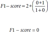
AUC is referred to as Area Under the Curve, i.e., the amount of area which is under the line (linear or nonlinear) [33]. ROC means Receiver Operating Characteristic; initially, it was used for differentiating noise from not noise, but in recent years, it is used very frequently in binary classification [3] Figure 3.7.
ROC gives the trade-off between TP and the FP where x-axis represents FPR and y-axis represents TPR. The total area of ROC is 1 unit because TPR and FPR value has range [0, 1] [33]. It can be analyzed that more the area under the curve better the model as it can differentiate between positive and negative class but AUC in ROC should be greater than 0.5 unit [3].
Figure 3.7 AUC-ROC curve.
If AUC of ROC = 1, then the binary classification model can perfectly classify the entire positive and negative class points correctly [29].
If AUC of ROC = 0, then the binary classifier is predicting all negative labels as positive labels, and vice versa [4].
If 0.5 < AUC of ROC < 1, then there is a high chance that the binary classification model can classify positive labels and negative labels. This is so because the classifier is able to differentiate between TPs and TNs than FNs and FPs [5]. If AUC of ROC = 0.5, then the classifier is not able to distinguish between positive and negative labels, i.e., the binary classification model is predicting random class for all the dataset [3].
In some book, the y-axis can be represented as Sensitivity which is known as TPR and the x-axis can be represented as Specificity which can be determined by 1 – FPR [3].
Steps to construct AUC-ROC:
- 1. Arrange the dataset on the basis on the predictions of probability in decreasing order.
- 2. Set the threshold as the ith row of the prediction (for first iteration, take first prediction; for second iteration, take second as the threshold).
- 3. Calculate the value of TPR and FPR.
- 4. Iterate through all the data points in the dataset and repeat steps 1, 2, and 3.
- 5. Plot the value of TPR (Sensitivity) and FPR (Specificity = 1 – FPR).
- 6. Select the model with maximum AUC.
The pseudo-code for the calculation of the AUC-ROC is as follows:
TPR = []
FPR = []
Sorted_predictions = sort(probability_prediction) For I in Sorted_predictions:
Threshold = I
TPR.append(Calculate TPR)
FPR.append(Calculate FPR)
Plot_AUC_ROC (TPR, FPR)
3.4.14 AUC - PRC
AUC is referred to as Area Under the Curve, i.e., the amount of area which is under the line (linear or nonlinear). PRC means Precision-Recall Curve; it is used very frequently in binary classification [33].
PRC gives the trade-off between precision and recall where the x-axis represents precision and y-axis represent recall. The total area of PRC is 1 unit because precision and recall value has range [0, 1] [33]. It can be clearly analyzed that more the area under the curve better the model as it can clearly differentiate between positive and negative class but AUC in PRC should be greater than 0.5 unit because of imbalance in the dataset as small change in prediction can show a drastic change in AUC-PRC curve [3] (Figure 3.8).
A binary classification model with correct predictions is depicted as a point at a coordinate of (1, 1). A skillful model is represented by a curve that bends toward a coordinate (1, 1) [5]. A random binary classification model will be a horizontal line on the plot with a precision that is proportional to the number of positive examples in the dataset. For a balanced dataset, this will be 0.5 [4]. The focus of the PRC on the minority class makes it an effective diagnostic for imbalanced binary classification models. Precision and recall make it possible to assess the performance of a classifier on the minority class [29]. PRCs are recommended for highly skewed domains where ROC curves may provide an excessively optimistic view of the performance [5].
Steps to construct AUC-PRC:
- 1. Arrange the dataset on the basis on the predictions of probability in decreasing order.
- 2. Set the threshold as the ith row of the prediction (for first, take 1 prediction; for second, take second as the threshold).
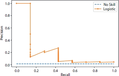
Figure 3.8 Precision-recall curve.
- 3. Calculate the value of precision and recall.
- 4. Iterate through all the data points in the dataset and repeat steps 1, 2, and 3.
- 5. Plot the value of precision and recall.
- 6. Select the model with maximum AUC.
The pseudo-code for the calculation of the AUC-ROC is as follows:
Precision = []
Recall = []
Sorted_predictions = sort(probability_prediction) For I in Sorted_predictions:
Threshold = I Precision.append(Calculate Precision) Recall.append(Calculate Recall)
Plot_AUC_PRC (Precision, Recall)
3.4.15 Derived Metric From Recall, Precision, and F1-Score
The micro average is the precision or recall of F1-score of classes.
The macro average is defined as the average of precision or recall of F1-score of classes (more than one class).
The weighted average is the weight associated with precision or recall or F1-score of the classes where we control the precision or recall or F1-score of the classes by giving importance to one class and penalizing the other class [48]. It is the improvised version of the macro average.
Since we have discussed confusion metric and metric related to it, for better understanding, let us solve one example where dataset consists of 460 samples from two classes.
3.4.16 Solved Examples
From Figure 3.9, i.e., confusion metric, we can deduce the following metrics:
TP = 200
FN = 60
FP = 20
TN = 180
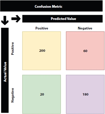
Figure 3.9 Confusion metric example.
So, here, we have all the information required for calculation of the metrics which are as follows:


3.5 Correlation
Correlation is defined as the relationship between two variable IV and DV; it ranges between [–1, 1], whereas –1 means highly negative correlation, i.e., increase in DV will tend to decrease in IV, or vice versa, 0 means no correlation, i.e., no relationship exists between IV and DV, and 1 means highly positive correlation, i.e., increase in DV will tend to increase in IV, or vice versa [16].
While in implementation, we use to set the threshold for both sides so that we can incorporate the IV which are highly correlated in terms of the absolute value of magnitude and then we process further to build the model [16]. Correlation estimation is done before building the model but, in some cases, where we have limitations like computing power and storage scarcity, we use correlation metric to justify our regression model by showing the relation between IV and DV. Below are the correlation metrics which are used widely to justify the model indirectly, i.e., justifies the model by justifying its predictors/features (X = IV and Y = DV, respectively) [15]:
3.5.1 Pearson Correlation
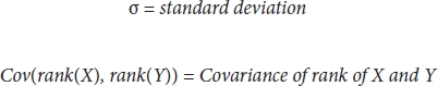
Pearson correlation is defined as the covariance of two variable normal-ized by the product of the standard deviation of the variables denoted by r. It measures a linear association between two variables—parametric correlation [14]. It is also known as the product-moment correlation coefficient between two variables IV and DV which ranges from [–1, 1] where 0 = no relation, 1 = positive relation, and –1 = negative relation, respectively [14].
Assumptions:
- 1. IV and DV are normally distributed.
- 2. Both IV and DV are continuous and as linearly related.
- 3. No outliers are present in the IV and DV (it affects the mean).
- 4. IV and DV are homoscedasticity (homogeneity of variance).
Formulae:
where
Steps of Pearson correlation:
- 1. Find the covariance of X and Y.
- 2. Find the standard deviation of X and Y.
- 3. Multiply the covariance of X and Y and divide by multiplication of the standard deviation of X and Y.
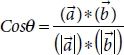
3.5.2 Spearman Correlation
Spearman correlation is a non-parametric test which is used to measure the association between the two variables [19]. It is equal to the Pearson correlation, and it is calculated as same as the Pearson correlation, but instead of the value, we use the rank of the variable denoted by ρ [21]. It ranges from [–1, 1] where 0 = no relation, 1 = positive relation, and –1 = negative relation, respectively.
Assumption:
- 1. IV and DV are linear and monotonous.
- 2. IV and DV are continuous and ordinal.
- 3. IV and DV are normally distributed.
Formulae:
where
Or,
where
N = Number of Samples
d = Difference in rank of X and Y
Steps of Spearman correlation:
- 1. Rank the variable X and Y.
- 2. Calculate the difference of the rank, i.e., d = R(x) – R(y).
- 3. Raise d to the power of 2 and perform summation.
- 4. Calculate N * (N – 1), where n is no of the variable.
- 5. Substitute the respective value in the below formulae.
- 6. (Optional) you can use the rank of the variable in Pearson’s formula and calculate the Spearman correlation.
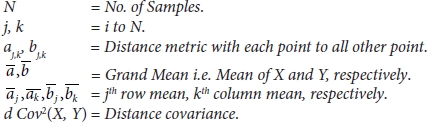
3.5.3 Kendall’s Rank Correlation
It is a non-parametric measure of the relationship between the columns of the ranked data. It is preferred over Spearman correlation because of the low GES (gross error sensitivity) and the asymptotic variance [19, 23]. It ranges from [–1, 1] where 0 = no relation, 1 = positive relation, and –1 = negative relation, respectively.
Assumption:
- 1. IV and DV are linear and monotonous.
- 2. IV and DV are continuous and ordinal.
- 3. IV and DV are normally distributed.
Formulae:

where
N = Number of Samples
C = Number of Concordant Pair
D = Number of Discordant Pair
A quirk test can produce a negative coefficient, hence making the range between [–1, 1], but when we are using ranked data, the negative value does not mean much. Several version of tau correlations exists such as τ A, τ B, and τ C. τ A is used with a squared table (no. of row == no. of columns), and τ C for rectangular columns [24].
Briefly, concordant [23] means ranks are ordered in same order irrespective of the rank (X increases, Y also increases) and discordant [23] (X increases, Y also decreases) means ranks are ordered in opposite way irrespective of rank.
Steps of Kendall’s rank correlation:
Steps to find concordant:
- 1. Take any column X or Y.
- 2. For the first value in the selected count no. of values in the respective column starting from the next row which is greater than the selected value in row. Suppose you are calculating a concordant for ith row, so you will take values from (i+1)th row from the Interview column.
Steps to find discordant:
- 1. Take any column X or Y.
- 2. For first value in the selected feature, i.e., Interviewer 2, count no of value in the respective column starting from next row which is smaller than the selected value in row. Suppose you are calculating a concordant for ith row, so you will take values from (i+1)th row from the interview column.
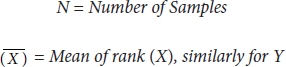
3.5.4 Distance Correlation
Distance correlation is used to test the relation between the IV and DV which are linear or nonlinear, in contrast with the Pearson which applies to only linear related data [51]. Statistical test of dependence can be performed with a permutation test. It ranges from [0, 1] where 0 = no relation, 1= positive relation, and –1 = negative relation, respectively.
Steps of distance correlation:
- 1. Calculate the distance metric of X and Y.
- 2. Calculate doubly center for X and Y each element.
- 3. Multiply the doubly center of X and Y for each term take the summation and finally divide by N raised to 2.
Formulae:
Or, for two random variables,
where
3.5.5 Biweight Mid-Correlation
This type of correlation is median base instead of the traditionally mean base, also known as bicorr, which measures similarity between samples [50]. It is less affected by outliers because it is independent of mean. It ranges from [0, 1] where 0 = no relation, 1 = positive relation, and –1 = negative relation, respectively.
Assumptions:
- 1. IV and DV are normally distributed.
- 2. Both IV and DV are continuous or ordinal.
Formulae:

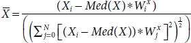
Finally,
where
3.5.6 Gamma Correlation
It is the measurement of rank correlation equivalent to the Kendal rank correlation [49]. It is robust to outliers and denoted by gamma, i.e., γ. Its goal is to predict where new value will rank. It applies to data which are tied with their respective rank [50]. It ranges from [0, 1] where 0 = no relation, 1 = positive relation, and –1 = negative relation, respectively.
Formulae:
where
Nc = Number of Concordant Pair.
Nd = Number of Discordant Pair.
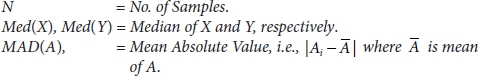
3.5.7 Point Biserial Correlation
This type of correlation is used to calculate the relationship between the dichotomous (binary) variable and continuous variable works well then IV and DV are linearly dependent [53]. It is same as the Pearson correlation; the only difference is that it works with dichotomous and continuous variable and denoted by rpb [53]. It ranges from [0, 1] where 0 = no relation, 1 = positive relation, and –1 = negative relation, respectively.
Assumptions:
- 1. IV and DV are normally distributed, i.e., mean = 0 and variance = 1 or bell-shaped curve.
- 2. Anyone of them IV or DV should be continuous or ordinal and another should be dichotomous.
Formulae:
Or,
where
M0 = Mean of data with group 0.
M1 = Mean of data with group 1.
Sn = Standard deviation of Continuous data.
p = Proportion of cases in group 0 ![]() .
.
q = Proportion of cases in group 1 ![]() .
.
n = Total Number of observation.
no = Number of observation in group 0.
n1 = Number of observation in group 1.
3.5.8 Biserial Correlation
Biserial correlation is almost the same as point biserial correlation, but one of the variables is dichotomous ordinal data and has an underlying continuity and denoted by rb [53]. It ranges from [0, 1] where 0 = no relation, 1 = positive relation, and –1 = negative relation, respectively.
Assumptions:
- 1. IV and DV are normally distributed.
- 2. Anyone of them IV or DV should be ordinal which has underlying continuity, and another should be dichotomous.
Formulae:
where
Yo = Mean Score of data point at X = 0.
Y1 = Mean Score of data point at X = 1.
p = Proportion of data pairs for X = 1.
q = Proportion of data pairs for X = 0.
σy = Population standard deviation.
Y = Height of standard Normal Distribution.
3.5.9 Partial Correlation
The partial correlation measures the strength of correlation between the variables by controlling one or more variables [51]. Like if the dataset has 5 IV, then we calculate correlation with 1 IV and DV and then we calculate the correlation between 2 IV and DV and so on. Therefore, some discrepancies are there when we compare t and p-value from other correlation methods [52].
3.6 Natural Language Processing (NLP)
Evaluation of the NLP model is a little tricky to evaluate because the output of these model is text/sentence/paragraph. So, we have to check the syntactical, semantic, and the context of the output of the model [41]; so, we use different types of techniques to evaluate these models, some of the metric based on word levels, sentence level, and so on. Let us have some basic intuition about NLP models. NLP deals with Natural Language— humans use to communicate with each other, i.e., it deals with the text data [49]. We all know that ML models take input as numerical value, i.e., numeric tensor, and give numeric output. So, we need to convert these text data into numerical format. For this, we have various pre- processing techniques such as Bog of Words, Word2vector, Doc2vector, Term Frequency (TF), Inverse Term Frequency (ITF), and Term Frequency-Inverse Term Frequency (TF-IDF) [41], or you can do manually by various techniques. For now, you do not need to get carried away just assume that text has been converted by some algorithm or method into numerical value and vice versa.
3.6.1 N-Gram
In ML, gram is referred as a word and N is an integer. So, N-gram refers to the count of words in a sentence [49]; if a sentence is made-up of 10 words, then it will be called as 10-gram. It is used to predict the probability of the next word in the sentence depending how the model is trained, i.e., om Bigram trigram and so on using the probability of occurrence of the word related to its previous word.
N – Gram = N (Natural) + Gram (word)
Reference Sentence: I am a human.
So,
1 – Gram (UniGram): I, am, a, human.
2 – Gram (BiGram): I, am, am a, a human.
3 – Gram: (TriGram) I am a, am a human.
Similarly, we can group the words in a sentence according to N-Gram. and we predict the next word in the sentence irrespective of the context.
3.6.2 BELU Score
BELU stands for the Bi-Lingual Evaluation Understudy—it was invented to evaluate the language translation from one language to another [41, 49].
Steps to calculate BELU are as follows:
Step 1: From the predicted word, assign the value 1 if the word matches with the training set else assign 0.
Step 2: Normalize the count so that it has range of [0–1], i.e., total count/no. of words in reference sentence.
The below example shows how the BELU score of the predicted sentence is calculated by implementing the above-mentioned steps.
Original sentence: A red car is good.
Reference sentence 1: A red car is going.
BELU score: (1 + 1 + 1 + 1 + 0)/5 = 4/5
Reference sentence 2: A red car is going fast and looks good.
BELU score: (1 + 1 + 1 + 1 + 1)/5 = 5/5 = 1
Reference sentence 3: On the road the red car is good.
BELU score: (1 + 1 + 1 + 1 + 1)/5 = 5/5 = 1
As we can see from the above example, that Reference Sentence 2 and Reference Sentence 3 have BELU score of 1 respective but the meaning of them were completely different from the original sentence. Hence, BELU score did not consider the meaning of the sentence; it just took the present of the word in the respective sentence to calculate the BELU score; to counter this problem, BELU score with N-Gram was introduced which is discussed below.
3.6.2.1 BELU Score With N-Gram
BELU score with N-Gram is almost same as the BELU score but we use combination of the word, i.e., N-Gram to calculate the BELU score [41]. BELU score with N-Gram also limits the number of times the word has been used in the document or in sentence which helps us to avoid unnecessary repetition of words. Finally, we try to mitigate the loss if the detail in the predicted sentence by introducing brevity penalty, i.e., we try to keep the predicted output from the model to be greater than the reference sentence [41].
where brevity penalty = 1, if length of output sentence predicted by the NLP model is greater than the length of the shortest sentence referenced, i.e., length of the shortest reference sentence in the training set.
for the else part.
BELU score is not able to consider the meaning, structure as well as it cannot handle morphological rich language [41].
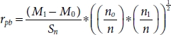
3.6.3 Cosine Similarity
It is a metric which is used to define the similarity between two documents earlier commonly used approach which was used to match similar documents is based on counting the maximum number of common words between the documents [47]. But this approach has flaws, i.e., the size of the document increases, the number of common words tends to increase even if the two documents are unrelated. As a result, cosine came into existence which removed the flaws of the count the common word or the Euclidean distance [47].
Mathematically, cosine is the measurement of the angle between two vector projected in a multi-dimensional space. In this context with the NLP, the two vectors arrays of word counts are associated with the two documents. Cosine calculates the direction instead of the magnitude, whereas the Euclidean distance calculates magnitude [47, 49]. It is advantageous because even if the two similar documents are far apart by the Euclidean distance because of the size (like, the word “cricket” appeared 50 times in one document and 10 times in another), they could still have a smaller angle between them. The smaller the angle, the higher the similarity.
Formulae:
where
Let us assume that we have three documents, and after tokenization, we found the below information from Table 3.4 and we have project its cosine similarity on 3D plane in Figure 3.10.
Table 3.4 Document information and cosine similarity.
| Document name | Number of similar words | Cosθ |
| Document 1 and Document 2 | 70 | 0.15 |
| Document 2 and Document 3 | 57 | 0.23 |
| Document 1 and Document 3 | 27 | 0.77 |
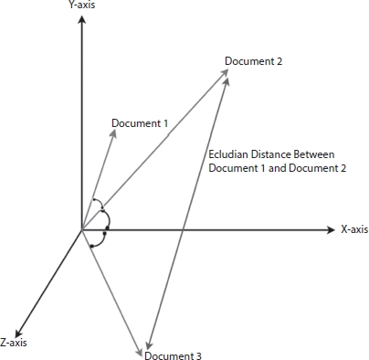
Figure 3.10 Cosine similarity projection.
From Table 3.4 and Figure 3.10, Document 1 and Document 2 as well as Document 2 and Document 3 have more similar word, i.e., 70 and 57 words, respectively; hence, the value of Cosθ will be less, i.e., 0.15 and 0.23, respectively; as a result, when we will project these documents in 3D plane, they will be close to each other and hence they will have more similarity. If we consider Document 1 and Document 3, we can see from the table that number of similar word is 27; as a result, Cos(theta) is close to 1, i.e., 0.77, and when we project these information in 3D plane, the orientation of the Document 1 and Document 3 will be far from each other, as shown in Figure 3.10. So, we can conclude that smaller the value of Cosθ, documents are similar. Cosθ lies between 0 and 1; hence, Cosθ close to 0 similarity increases and vice versa.
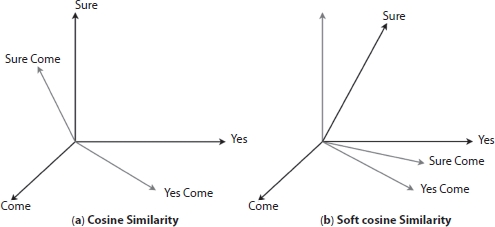
Figure 3.11(a) Cosine similarity. (b) Soft cosine similarity.
If you have another set of documents on a completely different topic, say “food”, you want a similarity metric that gives higher scores for documents belonging to the same topic and lower scores when comparing docs from different topics. So, we need to consider the semantic meaning, i.e., words similar in meaning should be treated as similar [49]. For example, “President” vs. “Prime minister”, “Food” vs. “Dish”, “Hi” vs. “Hello” should be considered similar. For this, converting the words into respective word vectors and then computing the similarities can address this problem by soft cosine [25, 49]. Soft cosine is very useful when you have to compare the semantic similarity of the word. Figure 3.11.a represents the cosine similarity which is close to 1, i.e., they are not similar, but if we consider Figure 3.11.b which is close to 0, i.e., they are similar hence it considers semantic meaning of the words before calculating the similarity.
3.6.4 Jaccard Index
Jaccard index is defined as the Jaccard similarity coefficient, which is used to understand the similarity or diversity between two finite sample sets [44] and have range [0, 1]. If the data is missing in the sample set, then it is replaced by zero, mean or the missing data is produced by the k-nearest algorithm or expectation-maximization algorithm (EM algorithm) [20, 36].
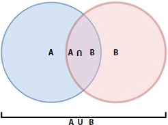
Figure 3.12 Intersection and union of two sets A and B.
Formulae: By referring Figure 3.12 mathematically Jaccard Index can be defined as:
By substituting Equation (3.131) in Equation (3.132), then we will get
3.6.5 ROUGE
ROGUE stands for Recall-Oriented Understudy for Gisting Evaluation, which is collection of the metric for evaluation of the transcripts produced by the machine, i.e., generation of the text and the text generation by NLP model based on overlapping of N-grams [25].
The metrics which are available in ROGUE are as follows:
ROUGE-N: overlap of N-grams between the system and reference summaries.
ROUGE-1: refers to the overlap of unigram (each word) between the system and reference summaries.
ROUGE-2 refers to the overlap of bigrams between the system and reference summaries.
ROUGE-L: Longest Common Subsequence (LCS)–based statistics. Longest common subsequence problem takes into account sentence-level structure similarity naturally and identifies the longest co-occurring in sequence n-grams automatically.
ROUGE-W: Weighted LCS-based statistics that favors consecutive LCSes. ROUGE-S: Skip-bigram–based co-occurrence statistics. Skip-bigram is any pair of words in their sentence order.
ROUGE-SU: Skip-bigram plus unigram-based co-occurrence statistics.
3.6.6 NIST
NIST stands for National Institute of Standard and Technology situated in the US. This metric is used to evaluate the quality of text produced by the ML/DL model [49]. NIST is based on BELU score, which calculates n-gram precision by giving equal weight to each one, whereas NIST calculates how much information is present in N-gram, i.e., when model produces correct n-gram and the n-gram is rare, then it will be give more weight. In simple words, we can say that more weight or credit is given to the n-gram which is correct and rare to produce as compared to the n-gram which is correct and easy to produce [49].
Example, if the trigram “task is completed” is correctly matched, then it will receive lower weight as compared to the correct matching of trigram “Goal is achieved”, as this is less likely to occur.
3.6.7 SQUAD
SQUAD refers to the Stanford Question Answering Dataset [41]. It is the collection of the dataset which includes the Wikipedia article and questions related to it. The NLP model is trained on this dataset and tries to answer the questions [41]. SQUAD consists of 100,000+ question-answer pairs and 500+ articles from Wikipedia [49]. Though it is not defined as a metric it is used to judge the model usability and predictive power to analyze the text and answer questions which is very crucial in NLP applications like a chatbot, voice assistance, and chatbots.
The key features of SQUAD are as follows:
- 1. It is closed dataset, i.e., questions and answers are always a part of the dataset and in series like Name of the spacecraft was Apollo 11.
- 2. Most of the answers, i.e., almost 75% are less than or equal to 4.
- 3. Finding an answer can be simplified as finding the start index and the end index of the context that corresponds to the answers
3.6.8 MACRO
MACRO stands for Machine Reading Comprehension Dataset similar to SQUAD; MACRO also consists of 1,1010,916 anonymized questions collected from Bing’s Query Log’s with answers purely generated by humans [49]. It also contains human written 182,669 question answers—extracted from 3,563,535 documents.
NLP models are trained on this dataset and try to perform the following tasks:
- 1. Answer the question based on the passage. As mentioned above, the question can be an anonymous or original question. So, custom or generalized word2vec, doc2vector, or Gloves are required to train the model—Question Answering
- 2. Rank the retrieved passage given in the question—Passage Ranking.
- 3. Predict whether the question can be answered from the given set of passages, if yes, then extract and synthesize the predicted answer like a human.
3.7 Additional Metrics
There are few metrics which are used rarely, or they are derived from the other metric used unfrequently are listed below:
3.7.1 Mean Reciprocal Rank (MRR)
Mean Reciprocal Rank is a measure to evaluate systems that return a ranked list of answers to queries. This is the simplest metric of the three. It tries to measure “Where is the first relevant item?”. It is closely linked to the binary relevance family of metrics. For a single query, the reciprocal rank where rank is the position of the highest-ranked answer. If no correct answer was returned in the query, then the reciprocal rank is 0 [58].
This method is simple to compute and is easy to interpret. This method puts a high focus on the first relevant element of the list. It is best suited for targeted searches such as users asking for the “best item for me”. Good for known-item search such as navigational queries or looking for a fact. The MRR metric does not evaluate the rest of the list of recommended items. It focuses on a single item from the list. It gives a list with a single relevant item just as much weight as a list with many relevant items [58]. It is fine if that is the target of the evaluation. This might not be a good evaluation metric for users that want a list of related items to browse. The goal of the users might be to compare multiple related items.
Formulae:
3.7.2 Cohen Kappa
Kappa is similar to accuracy metric score, but it considers the accuracy that would have been happened through random prediction [54]. It can be also defined as how the model exceeded random prediction in terms of the accuracy metric.
3.7.3 Gini Coefficient
As we have discussed AUC-ROC curve in confusing metric section (3.4.13), Gini coefficients is derived from AUC-ROC curve; it is an indicator which shows how well the model outperforms the random prediction [54]. It is also used to explain how the model exceeded random model prediction in terms of AUC-ROC curve.
3.7.4 Scale-Dependent Errors
Scale-dependent errors, such as mean error (ME) mean percentage error (MPE), mean absolute error (MAE), and root mean squared error (RMSE), are based on a set scale, which for us is our time series, and cannot be used to make comparisons that are on a different scale [55]. For example, we would not take these error values from a time series model of the sheep population in Scotland and compare it to corn production forecasts in the United States.
Mean Error (Me) shows the average of the difference between actual and forecasted values.
Mean Percentage Error (Mpe) shows the average of the percent difference between actual and forecasted values. Both the ME and MPE will help indicate whether the forecasts are biased to be disproportionately positive or negative [55].
Root Mean Squared Error (Rmse) represents the sample standard deviation of the differences between predicted values and observed values [56]. These individual differences are called residuals when the calculations are performed over the data sample that was used for estimation and are called prediction errors when computed out-of-sample. This is a great measurement to use when comparing models as it shows how many deviations from the mean the forecasted values fall.
Mean Absolute Error (MAE) takes the sum of the absolute difference from actual to forecast and averages them [57]. It is less sensitive to the occasional very large error because it does not square the errors in the calculation.
3.7.5 Percentage Errors
Percentage errors, like Mape, are useful because they are scale-independent [49], so they can be used to compare forecasts between different data series, unlike scale-dependent errors. The disadvantage is that it cannot be used in the series and has zero values.
Mean Absolute Percentage Error (Mape) is also often useful for purposes of reporting [49], because it is expressed in generic percentage terms it will make sense even to someone who has no idea what constitutes a “big” error in terms of dollars spent or widgets sold.
3.7.6 Scale-Free Errors
Scale-free errors were introduced more recently to offer a scale- independent measure that does not have many of the problems of other errors like percentage errors.
Mean Absolute Scaled Error (MASE) is another relative measure of error that applies only to time series data. It is defined as the mean absolute error of the model divided by the mean absolute value of the first difference of the series [49]. Thus, it measures the relative reduction in error compared to a naive model. Ideally, its value will be significantly less than 1 but is relative to comparison across other models for the same series. Since this error measurement is relative and can be applied across models, it is accepted as one of the best metrics for error measurement.
3.8 Summary of Metric Derived from Confusion Metric
Suppose we have a confusion metric as shown above in Figure 3.13, and by taking this as an example, we can derive a few more metrics mentioned in Table 3.5.
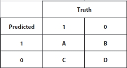
Figure 3.13 Confusion metric.
Table 3.5 Metric derived from confusion metric.
| Metric | Formulae | Interpretation |
| Sensitivity | What percentage of all 1 was correctly predicted? | |
| Specificity | What percentage of all 0 was correctly predicted? | |
| Prevalence | Percentage of true 1’s in the sample | |
| Detection Rate | Correctly predicted 1 as a percentage of entire samples. | |
| Detection | What percentage of full sample was | |
| Prevalence | predicted as 1? | |
| Balanced Accuracy | A balance between correctly predicting 1 and 0. | |
| Youden's Index |  | Similar to balance accuracy |
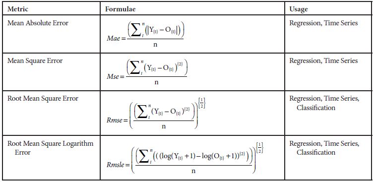
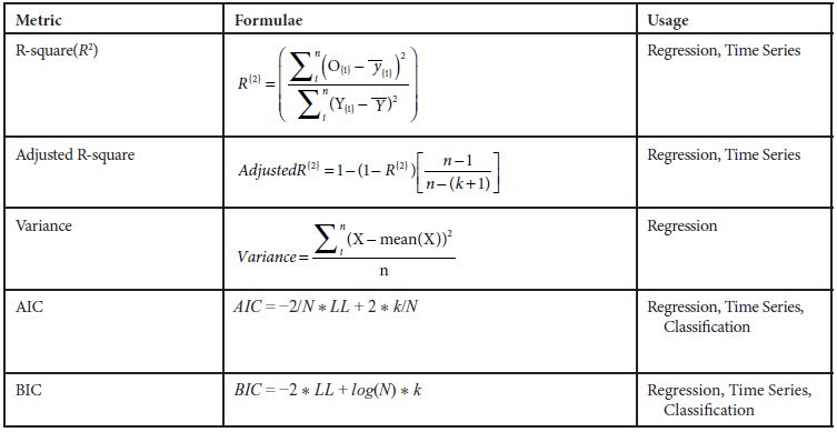
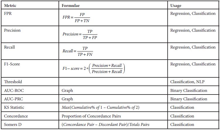
3.9 Metric Usage
Table 3.6 Metric usage.

3.10 Pro and Cons of Metrics
Table 3.7 shows the pro and cons of Metrics.
Table 3.7 Metric pros and cons.
| Metric | Pros | Cons |
| Mean Absolute Error | Avg. of absolute error | Not robust to outliers |
| Mean Square Error | Robust to outliers | Punishes error equally |
| Root Mean Square Error | Root enables it to show large number of deviation, punishes large error severely. | Affected by outliers |
| Root Mean Square Logarithm Error | Punishes large errors severely. | Affected by outliers, equivalent to Rmse |
| R-square (R2) | Compare the trained model with base model | Does not take account of usefulness of the features |
| Adjusted R-square (R2) | Take account of usefulness of the features | Dependent on R-square |
| Variance | Calculates Homogeneity of Nodes | Affected by outliers |
| AIC | Penalizes the model based on complexity | Dependent on Likelihood of the model |
| BIC | Penalizes the model based on complexity | Does not take account of the usefulness of the features |
| Accuracy | Calculates correctly predicted labels | Does not take account of the imbalance dataset |
| TPR | Proportional to goodness of model | Take account of the imbalance dataset |
| FNR | Indirectly proportional to goodness of model | Take account of the imbalance dataset |
| TNR | Proportional to goodness of model | Take account of the imbalance dataset |
| FPR | Indirectly proportional to goodness of model | Take account of the imbalance dataset |
| F1-Score | Takes account of Precision and Recall | Lacks interpretability |
| N-Gram | Split the word into N- integers | Does not consider the semantic nature of the sentence |
| Cosine | 3D-vector representation of the word | Does not consider the semantic nature of the sentence |
| Soft-Cosine | 3D-vector representation of the word, with semantic representation | Computational Expensive |
3.11 Conclusion
Model evaluation is one of the trending as well as vast topics in ML because it involves indepth understanding of the models along with data-set and objective. As we can see in Table 3.6, there is no concrete rule which states that the particular metric should be used with this type of dataset and model. Thus, choice of metric is totally dependent on the model, dataset, and our use case. In this chapter, in model evaluation, I have covered metrics which are widely used in Regression Classification, NLP, and Reinforcement Learning model theoretically but it is always suggested to have in-depth knowledge of the metric, which optimizes the model. We are just stepping into the era of Machine General Intelligence and knowing correct metrics always helps to optimize the model and validate the result of the problem statement easily.
References
1. Chawla, Nitesh & Japkowicz, Nathalie & Kołcz, Aleksander. (2004). Editorial: Special Issue on Learning from Imbalanced Data Sets. SIGKDD Explorations.
6. 1–6. 10.1145/1007730.1007733.
2. Tom Fawcett,An introduction to ROC analysis, Pattern Recognition Letters, 27, 8, 2006, pp. 861-874, ISSN 0167-8655, https://doi.org/10.1016/j.patrec.2005.10.010.
3. Davis, J. and Goadrich, M., The relationship between precision-recall and ROC curves, in: Proc. of the 23rd International Conference on Machine Learning, pp. 233–240, 2006.
4. Drummond, C. and Holte, R.C., Cost curves: An Improved method for visu-alizing classifier performance. Mach. Learn., 65, 95–130, 2006.
5. Flach, P.A., The Geometry of ROC Space: understanding Machine Learning Metrics through ROC Isometrics, in: Proc. of the 20th Int. Conference on Machine Learning (ICML 2003), T. Fawcett and N. Mishra (Eds.), pp. 194– 201, AAAI Press, Washington, DC, USA, 2003.
6. Garcia, V., Mollineda, R.A., Sanchez, J.S., A bias correction function for classification performance assessment in two-class imbalanced problems. Knowledge-Based Syst., 59, 66–74, 2014. Int. J. Data Min. Knowl. Manage. Process (IJDKP), 5, 2, 10, March 2015.
7. Garcia, S. and Herrera, F., Evolutionary training set selection to optimize C4.5 in imbalance problems, in: Proc. of 8th Int. Conference on Hybrid Intelligent Systems (HIS 2008), IEEE Computer Society, Washington, DC, USA, pp. 567–572, 2008.
8. Garcia-Pedrajas, N., Romero del Castillo, J.A., Ortiz-Boyer, D., A cooperative coevolutionary algorithm for instance selection for instance-based learning. Mach. Learn., 78, 381–420, 2010.
9. Gu, Q., Zhu, L., Cai, Z., Evaluation Measures of the Classification Performance of Imbalanced Datasets, in: Z. Cai, et al., (Eds.), ISICA 2009, CCIS 51, pp. 461–471 Springer-Verlag, Berlin, Heidelberg, 2009.
10. Han, S., Yuan, B., Liu, W., Rare Class Mining: Progress and Prospect, in: Proc. of Chinese Conference on Pattern Recognition (CCPR 2009), pp. 1–5, 2009.
11. Hand, D.J. and Till, R.J., A simple generalization of the area under the ROC curve to multiple class classification problems. Mach. Learn., 45, 171–186, 2001.
12. Hossin, M., Sulaiman, M.N., Mustapha, A., Mustapha, N., A novel performance metric for building an optimized classifier. J. Comput. Sci., 7, 4, 582– 509, 2011.
13. Hossin, M., Sulaiman, M.N., Mustapha, A., Mustapha, N., Rahmat, R.W., OAERP: a Better Measure than Accuracy in Discriminating a Better Solution for Stochastic Classification Training. J. Artif. Intell., 4, 3, 187–196, 2011.
14. Hossin, M., Sulaiman, M.N., Mustapha, A., Mustapha, N., Rahmat, R.W., A Hybrid Evaluation Metric for Optimizing Classifier, in: Data Mining and Optimization (DMO), 2011 3rd Conference on, pp. 165–170, 2011.
15. Huang, J. and Ling, C.X., Using AUC and accuracy in evaluating learning algorithms. IEEE Trans. Knowl. Data Eng., 17, 299–310, 2005.
16. Huang, J. and Ling, C.X., Constructing new and better evaluation measures for machine learning, in: Proc. of the 20th International Joint Conference on Artificial Intelligence (IJCAI 2007), R. Sangal, H. Mehta and R. K. Bagga (Eds.), Morgan Kaufmann Publishers Inc., San Francisco, CA, USA, pp. 859– 864, 2007.
17. Japkowicz, N., Assessment metrics for imbalanced learning, in: Imbalanced Learning: Foundations, Algorithms, and Applications, pp. 187–210, Wiley IEEE Press, 2013.
18. Joshi, M.V., On evaluating performance of classifiers for rare classes, in: Proceedings of the 2002 IEEE Int. Conference on Data Mining (ICDN 2002) ICDM’02, IEEE Computer Society, Washington, D. C., USA, pp. 641–644, 2002.
19. Kohonen, T., Self-Organizing Maps, 3rd ed., Springer-Verlag, Berlin Heidelberg, 2001.
20. Kuncheva, L.I., and Bezdek, J.C., Nearest Prototype Classification: Clustering, Genetic Algorithms, or Random Search? IEEE Trans. Syst. Man Cybern.-Part C: Appl. Rev., 28, 1, 160–164, 1998.
21. Lavesson, N. and Davidsson, P., Generic Methods for Multi-Criteria Evaluation, in: Proc. of the Siam Int. Conference on Data Mining, SIAM Press, Atlanta, Georgia, USA, pp. 541–546, 2008.
22. Lingras, P. and Butz, C.J., Precision and recall in rough support vector machines, in: Proc. of the 2007 IEEE Int. Conference on Granular Computing (GRC 2007), IEEE Computer Society, Washington, DC, USA, pp. 654–654, 2007.
23. MacKay, D.J.C., Information, Theory, Inference and Learning Algorithms, Cambridge University Press, Cambridge, UK, 2003.
24. Mitchell, T.M., Machine Learning, MacGraw-Hill, USA, 1997.
25. Prati, R., Batista, G., Monard, M., A survery on graphical methods for classification predictive performance evaluation. IEEE Trans. Knowl. Data Eng., 23, 1601–1618, 2011.
26. Provost, F., Domingos, P. Tree Induction for Probability-Based Ranking. Machine Learning 52, 199–215 (2003). https://doi.org/10.1023/A:1024099825458
27. Rakotomamonyj, A., Optimizing area under ROC with SVMs, in: 1st Int. Workshop on ROC Analysis in Artificial Intelligence (ROCAI 2004), J. Hernandez-Orallo, C. Ferri, N. Lachiche and P. A. Flach (Eds.), Valencia, Spain, pp. 71–80, 2004.
28. Ranawana, R. and Palade, V., Optimized precision-A new measure for classifier performance evaluation, in: Proc. of the IEEE World Congress on Evolutionary Computation (CEC 2006), pp. 2254–2261, 2006.
29. Rosset, S., Model selection via AUC, in: Proc. of the 21st Int. Conference on Machine Learning (ICML 2004), C.E. Brodley (Ed.), p. 89, ACM, New York, NY, USA, 2004. Int. J. Data Min. Knowl. Manage. Process (IJDKP), 5, 2, 11, March 2015.
30. Skalak, D.B., Prototype and feature selection by sampling and random mutation hill climbing algorithm, in: Proc. of the 11th Int. Conference on Machine Learning (ICML 1994), W.W. Cohen and H. Hirsh (Eds.), pp. 293–301, Morgan Kaufmann, New Brunswick, NJ, USA, 1994.
31. Marina Sokolova, Guy Lapalme, A systematic analysis of performance measures for classification tasks, Information Processing & Management, 45, 4, 427–437, 2009, ISSN 0306-4573, https://doi.org/10.1016/j.ipm.2009.03.002.
32. Tan, P.N., Steinbach, M., Kumar, V., Introduction to Data Mining, Pearson Addison Wesley, Boston, USA, 2006.
33. Vuk, M. and Curk, T., ROC curve, lift chart and calibration plot. Metodološki zvezki, 3, 1, 89–108, 2006.
34. Hossin, Mohammad and M.N, Sulaiman. A Review on Evaluation Metrics for Data Classification Evaluations. International Journal of Data Mining & Knowledge Management Process. 5. 1–11, 2015.
35. Wilson, S.W., Mining oblique data with XCS, in: Advances in Learning Classifier Systems: Third Int. Workshop (IWLCS 2000), P.L. Lanzi, W. Stolzmann, S.W. Wilson (Eds.), pp. 283–290, Springer-Verlag, Berlin, Heidelberg, 2001.
36. Zhang, H. and Sun, G., Optimal reference subset selection for nearest neighbor classification by tabu search. Pattern Recognit., 35, 7, 1481–1490, 2002.
37. Senthilnathan, S., Relationships and Hypotheses in Social Science Research, https://ssrn.com/abstract=3032284 or http://dx.doi.org/10.2139/ssrn.3032284, New Zealand, 2017.
38. Smith, M.D., Handshoe, R., Handshoe, S., Kwan, O.L., Demaria, A.N., Comparative accuracy of two-dimensional echocardiography and Doppler pressure half-time methods in assessing severity of mitral stenosis in patients with and without prior commissurotomy. Circulation, 73, 1, Jan, 100–107, 1986.
39. Helen Victoria, A. and Maragatham, G., Automatic tuning of hyperparameters using Bayesian optimisation. Evolving System,12, 217–223, 2021.
40. Ramasamy, Pitchai & Babu, Ch & Perumal, Supraja & Challa, Mahesh. Cerebrum Tumor Segmentation of High Resolution Magnetic Resonance Images Using 2D-Convolutional Network with Skull Stripping. Neural Processing Letters, 53, 1–14, 2021.
41. Papineni, K.; Roukos, S.; Ward, T.; Zhu, W. J. (2002). BLEU: a method for automatic evaluation of machine translation (PDF). ACL-2002: 40th Annual meeting of the Association for Computational Linguistics. pp. 311–318. CiteSeerX 10.1.1.19.9416.
42. Tan, P.N., Steinbach, M., Kumar, V., Introduction to Data Minning, Addison-Wisely,, Pearnson, 97–114, 2005.
43. Chicco, D. and Jurman, G., The advantages of the Matthews correlation coefficient (MCC) over F1 score and accuracy in binary classification evaluation. BMC Genomics, 21, 1, 6-1–6-13, January 2020.
44. Sven Kosub, A note on the triangle inequality for the Jaccard distance, Pattern Recognition Letters, 120, pp. 36–38, 2019, ISSN 0167-8655, https://doi.org/10.1016/j.patrec.2018.12.007.
45. Joseph Lee Rodgers and W. ALan Nicewander, Thirteen Ways to Look at the Correlation Coefficient, The American Statistian, https://doi.org/10.1080/00031305.1988.10475524
46. D. G. Beech, 1962. "The Advanced Theory of Statistics. Volume 2, Inference and Relationship," Journal of the Royal Statistical Society Series C, Royal Statistical Society, 11(1), pp. 67–68, March.
47. Sirodovo, G., Gelbukh, A., Gomerz-Adorono, Pinto, D., Soft Simillarity and Soft Cosine Measure: Simillarity of the Feature in Space Model, 2014. arX-iv:1910.19129v2 [cs.IR] 31 Oct 2019.
48. Chicco, D. and Jurman, G., The Advantage of Mathew Correlation over F1 score and accuracy in Binary Classification. BMC Genomics, 2020.
49. Ming, T.K., Sammut, C., Webb, G., Encyclopedia of Machine Learning, Springer, 2017.
50. Damghani, M. and Babak, N.K., Measuring and Testing Independence by Correlation of Distances. Ann. Statist., 2007.
51. Dr. Arati Shah ,International Journal of Social Impact,Volume 5, Issue.
52. F. E. Croxton, D. J. Cowden, S. Klein, Prentice-Hall, Inc., Englewood Cliffs, N. J, “Applied General Statistics, Third Edition. 1967.” Journal of the American Statistical Association, 63(322), p. 738.
53. Linacre, J., The Expected Value of the Point Biserial Correlation, Rash Measurement Transaction, 2008.
54. Lehman, A., Jmp for Basic Univariate and Multivariate Statistic: A step by Step Guide, SAS Press, Cary, NC, 2005.
55. Supraja, P. and Jayashree, S., Optimised Neural Network for Spectrum Prediction Scheme in Cognitive Radio. Wirel. Pers. Commun., Springer, 24, 2, pp. 357–364.
56. Supraja, P., Gayatri, V.M., Pitchai, R., Optimise Neural Network for Spectrum Prediction using Genetic Algorithm in Cognitive Radio Network. Cluster Comput., Springer, 2017.
57. Shanthini, A., Vinodhini, Chandrasekaran, Supraja, P., A Taxonomy on Impact of Label Noise and Feature Noise using Machine Learning Techniques. Soft Comput., Springer, 2019, Pub Date : 2019-04-08,
58. Zhao Song and Wen Sun Efficient Model-free Reinforcement Learning in Metric Spaces in Machine Learning (cs.LG); Machine Learning (stat.ML) arXiv:1905.00475 [cs.LG]
59. Cowers, D.M.W., Evaluation, Evaluation From Precisin, ecall F-Measur To ROC, Informdmedness, Markedness and Correlation, Journal of Machine Learning Technologies, 2, 1, pp. 37–63, 2011.
Email: [email protected]