16
Simulation of Self-Driving Cars Using Deep Learning
Rahul M. K.*, Praveen L. Uppunda, Vinayaka Raju S., Sumukh B. and C. Gururaj
Department of Telecommunication Engineering, B.M.S College of Engineering, Bengaluru, India
Abstract
Self-driving cars have been a popular area of research for a few decades now. However, the prevalent methods have proven inflexible and hard to scale in more complex environments. For example, in developing countries, the roads are more chaotic and unstructured as compared to developed countries. Hence, the rule-based self-driving methodologies currently being used in developed countries cannot be applied to the roads in developing countries. Therefore, in this paper, a methodology of implementing self-driving is discussed which we propose that it will be better suited to more unstructured and chaotic environments.
As discussed, there are many approaches to solving self-driving, each with its advantages and disadvantages. In this paper, the concept of end-to-end learning with behavioral cloning applied for self-driving is discussed. We have experimented with two different neural network models, Convolutional Neural Network (CNN) and Multilayer Perceptron (MLP). Also, we have two different pre-processing pipelines, that is, with and without lane feature extraction. In the final result, the goal is to find the optimal combination of these methodologies to get the highest accuracy. It was found that the end-to-end learning CNN model without lane feature extraction gave the highest accuracy compared to the other combinations.
Keywords: Self-driving, behavioral cloning, end-to-end learning, CNN, MLP
16.1 Introduction
Most self-driving cars that are currently in the market are developed for structured roads, relying heavily on lane marking, handwritten rules for specific situations and road signs, etc. [2, 3]. This method has a profound disadvantage when it encounters the roads of developing countries, as they are not as structured and often do not have clear lane markings on the roads. Thus, using handwritten rules will fail in this scenario. To solve this problem, we propose the method of end-to-end learning with behavioral cloning. This is because the need of defining handwritten rules or policies in this methodology is eliminated. Although end-to-end learning has its disadvantages [11], we propose that it will perform better than the other methods in certain environments as described above.
Also, in this paper, six combinations of three different attributes are implemented to arrive at an optimal combination. The three different attributes are type of model (CNN/MLP), type of image processing pipeline (with/without lane feature extraction), and type of output (classification/regression).
16.2 Methodology
16.2.1 Behavioral Cloning
Behavioral cloning is a method that is used to capture human sub-cognitive skills. As a human subject performs the skill, his or her actions can be recorded along with the situation that gave rise to that action. This method can be used to construct automatic control systems for complex tasks for which classical control theory is inadequate. It can also be used for training [4, 10].
16.2.2 End-to-End Learning
End-to-end learning refers to training a complex learning system represented by a single model (usually a deep neural network) that represents the complete target system, bypassing the intermediate layers usually present in traditional pipeline designs [1].
In this end-to-end system, there are two main components, i.e., training component and the inference component [15]. The training component consists of recording all the actions of the human subject while he or she performs the task of driving, and then training the model using the collected data. In the inference component, the trained model drives the car, autonomously utilizing the knowledge of previously collected data.
16.3 Hardware Platform
In the current implementation, a physical prototype of the car is used to experiment different scenarios of processing, so that more practical insights of the model’s performance can be inferred, rather than using a software simulator. The prototype car is a custom-designed 3D printed 1:16 scale car with Ackerman steering which is shown in Figure 16.1. The actuators used are DC motors, and a servo motor is used to control the Ackerman steering. The processing unit used is a Raspberry Pi 3 Model B. A smartphone is used as a camera to capture images and feed it to the model. Also, a stand-alone PC is used to run certain models that require higher computing power. In this case, the images captured are transmitted from the car to the PC and the inference predictions are sent back from the PC wirelessly to the car over WIFI using the Robotic Operating System (ROS) framework.
ROS is the software stack used which acts as the communication middleware between different components in the system.

Figure 16.1 Prototype 1:16 scale car.
16.4 Related Work
One of the first implementations of behavioral cloning in self-driving was by ALVINN [5], which predicted driving parameters from road images and laser data. Nvidia has demonstrated end-to-end behavioral cloning in self-driving using deep CNNs, and surprisingly, this performed remarkably well and reintroduced the potential of end-to-end learning in self-driving [1]. The Nvidia model has gone through further iterations to result in a model that is nearly four times smaller, which enables it to be used in embedded systems [21]. Authors in [22] highlight which region of the image influences the resulting steering angle produced by end-to-end learning models. It was shown that end-to-end models accurately determined that lane markings had the most influence in the final steering angle produced by the model.
16.5 Pre-Processing
This section describes the pre-processing steps applied on the image before feeding it to the model. Figure 16.2 indicates the Image Processing Pipeline used.
16.5.1 Lane Feature Extraction
We assume that lane markings as the primary indicator needed for inferring driving parameters by the model. Therefore, in this step, only the lane features are extracted from the image and fed to the model. Lane features are extracted using classical computer vision algorithms such as Canny edge detector [6] and Hough transform [7, 13].

Figure 16.2 Image processing pipeline.
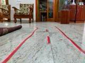
Figure 16.3 Original Image.
16.5.1.1 Canny Edge Detector
Canny edge detection is a technique to extract important structural information from different vision objects such as lane edges as shown in Figure 16.3. The canny output contains unwanted edge features also. Therefore, using a suitable mask, the unwanted regions are masked out. The resulting image Figure 16.4 ideally consists only of lane markings.
16.5.1.2 Hough Transform
Hough transform is the algorithm used to detect straight lines, circles, or other structures if their parametric equation is known. Here, it is used to highlight only the lane lines as shown in Figure 16.5. This method can give robust detection even under noise and partial occlusion [20].
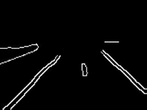
Figure 16.4 Canny edge output.
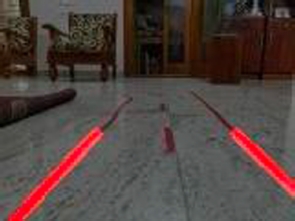
Figure 16.5 Hough lines overlaid on original image.
16.5.1.3 Raw Image Without Pre-Processing
In this method, we do not perform any pre-processing steps as described in the previous section. Instead, the raw images are fed directly to the model. The argument for this is based on the assumption that the model can make better internal learned representations of important features from the image not necessarily restricted to only lane features [8]. As stated earlier, in a situation where the roads do not contain any clear lane markings, the previous method fails, but in this method, the model can learn representations of features other than lane markings, e.g., identifying the contour of the road as a feature. Also, an argument can be made that the model can learn to extract lane features better than the previous method as the previous method uses classical methods which are very susceptible to lighting conditions, whereas a deep learning model can be more resilient to different lighting conditions [8, 9].
16.6 Model
In this implementation, we have experimented with two types of models, i.e., Convolutional Neural Network (CNN) [14] and Multilayer Perceptron (MLP) model. This section describes the architectures of the models.
16.6.1 CNN Architecture
The architecture that has been implemented is based on the model used by [1] which has been tweaked to obtain the optimal values for the model. The input size of the image is fixed to be 120 × 160. The CNN consists of five convolutional layers followed by two fully connected layers as depicted in Figure 16.6. Since the CNN requires a higher computing resource, it is not possible to run this on the Raspberry Pi 3 model B. Therefore, the images from the car are wirelessly transmitted to a stand-alone PC that is running the CNN. Then the stand-alone PC will infer from the image and transmit the driving parameters back to the car.
16.6.2 Multilayer Perceptron Model
Given its simplicity, the MLP model [19] was also considered since it has performed remarkably well in ALVINN [5]. Also, the added advantage of using MLP models is reduction in the requirement of computing resources, which makes it suitable for running it locally on the Raspberry Pi if needed. The disadvantage of MLP models is that, they are not very robust and cannot scale to different environments very easily and tend to overfit.
Similar to the previous model, the input image size is fixed to 120 × 160 pixels. It has four hidden layers with 50 neurons each and there a dropout of 0.1 in each layer as depicted by Table 16.1.
16.6.3 Regression vs. Classification
As stated before, we also experimented with type of output of the model, i.e., regression and classification. The aim is to find which among the two is better suited.

Figure 16.6 CNN model architecture.
Table 16.1 CNN architecture.
| Input image 120 x 160 | |
| Convolutional Layer 1 | 24@116 × 156 |
| Convolutional Layer 2 | 32@112 × 152 |
| Convolutional Layer 3 | 64@108 × 148 |
| Convolutional Layer 4 | 64@104 × 146 |
| Convolutional Layer 5 | 64 × 104 × 144 |
| Fully connected Layer 6 | 1 × 00 |
| Fully Connected Layer 7 | 1 × 50 |
| Output Layer | 6 (Classification) |
| 2 (Regression) | |
16.6.3.1 Regression
In regression, the output variable is continuous. The regression model used is defined by having two outputs, one for each driving parameter being steering angle and throttle. The range of steering angles is between [–M, M] degrees, where M is the maximum physical steering angle of the car and the throttle values are scaled in the range [0, 1]. The disadvantage or this is that the output is unbounded, and also regression models generally take longer to converge. The advantage of this is that the model is more precise in predicting the driving parameters.
16.6.3.2 Classification
In this method, the steering angles and throttle values are divided into discrete classes, by splitting the steering angle and throttle value intervals. For simplicity, the steering interval is divided into three classes, i.e., hard left, straight, and hard right. The throttle interval is divided into three classes, i.e., stationary, medium speed, and high speed. The disadvantage of using this method is that it is not precise and the probability error is high. However, the output is bounded between [–M, M] unlike regression. Also, classification models converge more easily.

Figure 16.7 Experimental track used for training and testing.
16.7 Experiments
As stated in Section 16.2, a 1:16 scale car has been built to test the models practically. To evaluate the models, a circuit/track was built to simulate a road like environment as shown in Figure 16.7. The car is driven by a human around the track keeping within the lanes to collect the training data initially. Using this, data eight different models were trained and the performance of these models on the track was tested.
16.8 Results
Here, the model is differentiated based on three attributes:
- i) CNN model/MLP model
- ii) Regression/classification
- iii) Feature extraction pre-processing/end-to-end learning
By the combination of these three attributes, eight different models are obtained that have been named Model 1 through Model 8. Each model is independently evaluated and, in the end, the aim is to obtain the model with the best overall accuracy.
The metrics chosen to evaluate each model are as follows:
- i) Accuracy
- ii) Categorical cross-entropy loss (for classification models)
- iii) Mean square error (for regression models)
Table 16.2 shows the definition of each model numbering from 1 through 8 each having a particular combination of the three attributes that we have chosen for comparison.
For classification models, the loss function used is the categorical cross-entropy loss. This loss function is obtained by the combination of SoftMax activation and cross-entropy loss which enables for it to be used for multi-class classification. In this implementation, there are three different classes, as mentioned in Section 16.6.3.2. This loss function treats each class with equal weightage, hence the training data needed to be normalized by having close to equal number of training samples for each class in order to avoid bias in the final model. In this case, there will be more training samples for driving straight than driving right or left, and hence it needed to be normalized.
For regression models, the loss function used is the mean squared error. This loss function is suitable for applications that have a continuous value as its output value. The mean error between the expected value and output value is squared so that it always remains positive.
Descriptions of results of some of the models which provided important insights and Table 16.3 contains the final results of each model.
From Figure 16.8, it can be seen that, as the number of epochs increases, the accuracy gradually increases.
By looking at the validation accuracy curve, it is clear that the validation accuracy also rises along with training accuracy; this is very desirable because it indicates that the network is not overfitting but is, in fact, learning only useful features of training data.
Table 16.2 Model definition.
| MLP | CNN | |||
| Classif. | Regres. | Classif. | Regres. | |
| End-to-End | Model 1 | Model 2 | Model 5 | Model 6 |
| FEP | Model 3 | Model 4 | Model 7 | Model 8 |
Classif., Classification; Regres., Regression; FEP, Feature Extraction Pre-processing
Table 16.3 Model results.
| Accuracy | Loss | MSE | ||||
| Train | Test | Train | Test | Train | Test | |
| Model 1 | 89% | 86% | 0.30 | 0.37 | _____ | |
| Model 2 | _____ | 300 | 280 | |||
| Model 3 | 84% | 80% | 0.38 | 0.54 | _____ | |
| Model 4 | _____ | 290 | 380 | |||
| Model 5 | 98% | 88% | 0.01 | 0.65 | _____ | |
| Model 6 | _____ | 100 | 300 | |||
| Model 7 | 98% | 75% | 0.01 | 2.2 | _____ | |
| Model 8 | _____ | 85 | 450 | |||
MSE, mean squared error.
From Figure 16.9, it can be observed that it is decreasing as the number of epochs increase. This is a typical behavior of a model that has generalized. Specifically observing the validation loss, it can be seen that it also decreases along with the training loss, but it has an oscillating behavior which may indicate that the network is finding it a bit more difficult to classify images it has not seen before. In our testing, the car was also able to traverse successfully on an entirely different track from which it was trained on, indicating that the model has satisfactorily generalized.

Figure 16.8 Accuracy vs. training time (hours) plot of Model 1 that uses classification method with MLP model without pre-processing.

Figure 16.9 Loss vs. training time (hours) plot of Model 1 that uses classification method with MLP model without pre-processing.
In regression models, the primary evaluation measure is the mean squared error. By observing Figure 16.10, it can be seen that both the training and validation MSE decreases with increase in the number of epochs. Observing the final MSE value and curve of the validation MSE, it can be seen that it has a lower value than the training MSE value. From this, it can be inferred that the MLP has not overfitted. This is very indicative that the MLP network has very successfully generalized and is able to predict the steering angles for images it has not seen before. However, the final error value is not desirable and there is room for improvement. In this case, the validation MSE is 280, meaning that there is an average error of 16.73° in the steering angle. However, an average error of 16.73° in the steering angle did not have a huge impact when the car was practically tested on the track; in fact, it was able to traverse the track successfully.

Figure 16.10 MSE vs. steps plot of Model 2 that uses classification method with MLP model without pre-processing.

Figure 16.11 MSE vs. steps plot of Model 8 that uses classification method with MLP model with pre-processing (feature extraction).
Looking at the MSE plot in Figure 16.11, it can be observed that training MSE decreases in a steady pace for every epoch; however, the validation error plateaus around a value of 450.
This is indicating that the model has not generalized suitably and has in fact completely overfitted on the training data. In our testing, the car was able to navigate around the track that it was trained on; however, the car failed to navigate around a new track other than the one it was trained on.
In observing the accuracy and loss scores shown in Figure 16.12, it can be seen that this model is a well-performing model. This model has the highest training and validation accuracies compared to the rest of the models.
Observing the loss values in Figure 16.13, it can be seen that the training loss has a very low value of 0.01 and validation loss is 0.65. However, by observing the loss plot, it can be seen that the training loss decreases along with an increase in the number of epochs whereas the validation loss increases. The inference that can be drawn from this is that the model is clearly overfitting. The fact of CNNs being very robust has worked to our disadvantage in this case, because by looking at some of the feature maps the CNN has derived, it can be seen that the CNN has overfitted on the background objects rather than extracting lane features. In practical testing of this car on the track, this model has performed the best compared to the rest of the models. The car was also able to traverse successfully in a different track from which it was trained on.

Figure 16.12 Accuracy vs. steps plot of Model 5 that uses classification method with CNN model without pre-processing.
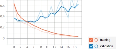
Figure 16.13 Loss vs. steps plot of Model 5 that uses classification method with model without pre-processing.
Considering all of the compiled results above, the best performing model is Model 5, which has the configuration:
- i) Convolutional Neural Network
- ii) End-to-End Learning
- iii) Classification Model
In all cases, this model performed consistently better compared to others. This result is not surprising since CNNs perform better when it comes to image classification [16].
Also, end-to-end learning has outperformed feature extraction preprocessing [17]. This means that the CNN has made better internal representations of lane features better than classical image processing algorithms [18]. This result is consistent with existing literature.

Figure 16.14 Input image given to CNN.
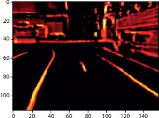
Figure 16.15 Feature map at second convolutional layer.

Figure 16.16 Feature map at the fifth convolutional layer.
Feature maps give an insight as to what the CNN actually sees and infers from for a given input image. Feature maps are obtained by convolving the filters derived by CNN with the input image Figure 16.14. These feature maps were derived using the model five configuration of CNN/classification/end-to-end. Also, techniques can be applied to get insights as to which part of the image the CNN gives more priority and weightage to calculate the final output [12].
In Figure 16.15, which is the output of the second convolutional layer, and it can be observed that at the second layer the CNN has extracted important edges from the image. It can be said that the second convolutional layer is performing an operation similar and analogous to the Canny edge detector.
In Figure 16.16, which is the output of the fifth convolutional layer, it can be observed that the final layer of the CNN has extracted only the lane features from the image and removed most of the background objects. It can be said that the fifth convolutional layer performs an operation similar and analogous to the Hough transform operation.
There are, however, limitations in using end-to-end learning for self-driving. The major limitation is the amount of training data required for the model to converge and reliably function in varied environments. The other limitation is that end-to-end systems are monoliths and do not have separate components to handle separate tasks, which makes it more difficult to train and debug specific functions within the model.
16.9 Conclusion
In this paper, the concept of behavioral cloning is explored for the task of self-driving. We have derived insights about the various methodologies used for implementing behavioral cloning, by comparing different models. These results indicate that end-to-end learning CNN model without any preprocessing steps such as lane extraction is the most optimal in terms of performance. This means that end-to-end learning has great potential to be used in environments where lane markings are absent or not clearly indicated.
References
1. Bojarski, M. et al., End to End Learning for Self-Driving Cars, arXiv: 1604.07316 [cs], Apr. 2016.
2. Birdsall, M., Google and ITE: The road ahead for self-driving cars. Inst. Transp. Eng. ITE J., 84, 5, 36–39, 2014.
3. Shalev-Shwartz, S., Shammah, S., Shashua, A., On a Formal Model of Safe and Scalable Self-driving Cars. ArXiv, abs/1708.06374, 2017.
4. Ghasemipour, S.K.S., Zemel, R., Gu, S., A Divergence Minimization Perspective on Imitation Learning Methods. Proceedings of the Conference on Robot Learning, in PMLR, vol. 100, pp. 1259–1277, 2020.
5. Pomerleau, D.A., Alvinn: An autonomous land vehicle in a neural network, in: Advances in neural information processing systems, pp. 305–313, 1989.
6. Daigavane, P.M. and Bajaj, P.R., Road lane detection with improved canny edges using ant colony optimization, in: 2010 3rd International Conference on Emerging Trends in Engineering and Technology, 2010, November, IEEE, pp. 76–80.
7. Saudi, A., Teo, J., Hijazi, M.H.A., Sulaiman, J., Fast lane detection with randomized hough transform, in: 2008 international symposium on information technology, 2008, August, vol. 4, IEEE, pp. 1–5.
8. Chen, Z. and Huang, X., End-to-end learning for lane keeping of self-driving cars. 2017 IEEE Intelligent Vehicles Symposium (IV), Los Angeles, CA, pp. 1856–1860, 2017.
9. Kim, J., Kim, J., Jang, G.J., Lee, M., Fast learning method for convolutional neural networks using extreme learning machine and its application to lane detection. Neural Networks, 87, 109–12, 2017.
10. Sammut, C. and Webb, G.I., (Eds.), Encyclopedia of machine learning, Springer, New York ; London, 2010.
11. Glasmachers, T., Limits of end-to-end learning, in: Proceedings of the Ninth Asian Conference on Machine Learning, vol. 77, pp. 17–32, Proceedings of Machine Learning Research, November 2017.
12. Selvaraju, R.R., Cogswell, M., Das, A., Vedantam, R., Parikh, D., Batra, D., Grad-CAM: Visual Explanations from Deep Networks via Gradient-Based Localization, in: 2017 IEEE International Conference on Computer Vision (ICCV), Oct. 2017, pp. 618–626.
13. Low, C.Y., Zamzuri, H., Mazlan, S.A., Simple robust road lane detection algorithm, in: 2014 5th International Conference on Intelligent and Advanced Systems (ICIAS), Jun. 2014, pp. 1–4.
14. Guo, T., Dong, J., Li, H., Gao, Y., Simple convolutional neural network on image classification. 2017 IEEE 2nd International Conference on Big Data Analysis (ICBDA), Beijing, pp. 721–724, 2017.
15. Bojarski, M. et al., Explaining How a Deep Neural Network Trained with End-to-End Learning Steers a Car, arXiv:1704.07911 [cs], Apr. 2017, Accessed: Dec. 05, 2020.
16. Driss, S.B., Soua, M., Kachouri, R., Akil, M., A comparison study between MLP and convolutional neural network models for character recognition, in: Real-Time Image and Video Processing 2017, May 2017, vol. 10223, p. 1022306.
17. Jiang, Y. et al., Expert feature-engineering vs. Deep neural networks: Which is better for sensor-free affect detection?, in: Artificial Intelligence in Education: 19th International Conference, AIED 2018, London, UK, June 27–30, 2018, Proceedings, Part I, Jan. 2018, pp. 198–211.
18. O’Mahony, N. et al., Deep learning vs. traditional computer vision, in: Advances in Computer Vision Proceedings of the 2019 Computer Vision Conference (CVC). pp. 128–144, Springer Nature Switzerland AG, Cham, 2020.
19. Ramchoun, H., Ghanou, Y., Ettaouil, M., Idrissi, M.A.J., ‘Multilayer Perceptron: Architecture Optimization and Training’. Int. J. Interact. Multimedia Artif. Intell., 4, Special Issue on Artificial Intelligence Underpinning, 26–30, 2016.
20. Assidiq, A.A., Khalifa, O.O., Islam, M.R., Khan, S., Real time lane detection for autonomous vehicles. 2008 International Conference on Computer and Communication Engineering, Kuala Lumpur, pp. 82–88, 2008.
21. Kocić, J., Jovičić, N., Drndarević, V., An end-to-end deep neural network for autonomous driving designed for embedded automotive platforms. Sensors, Basel, Switzerland, 9, 9, 2064, Jan. 2019.
22. Kim, J. and Canny, J., Interpretable Learning for Self-Driving Cars by Visualizing Causal Attention, in: 2017 IEEE International Conference on Computer Vision (ICCV), Oct. 2017, pp. 2961–2969.
- *Corresponding author: [email protected]