
12
Application of Machine Learning Algorithms With Balancing Techniques for Credit Card Fraud Detection: A Comparative Analysis
Shiksha
School of Computer Science and Mathematics, Liverpool John Moores University, Liverpool, United Kingdom
Abstract
This paper investigates the performance of the four supervised machine learning algorithms: logistic regression, support vector machine, decision tree, and random forest on the highly imbalanced ULB machine learning credit card fraudulent transaction dataset and a comparative analysis is performed. The major point that distinguishes this study from others is that this work is not only focused on the four supervised machine learning algorithms, rather than the permutation and combination of these methods with different balancing techniques are studied and analyzed for several evaluation metrics to obtain a better performance. In addition of the sampling techniques, one more method is used to balance the dataset by taking in account the balanced class weight at the modeling time. It is important to mention that the random forest with balanced class weight has shown the lowest false positive transactions with a value of only 3. The comparative results demonstrate that the random forest with SMOTE oversampling technique has output the best results in terms of all the selected metrics with accuracy of 99.92%, recall value of 81.08%, precision of 76.43%, F1-score of 78.69%, MCC of 0.79, AUC of 0.96, and AUPRC of 0.81.
Keywords: Supervised machine learning algorithms, logistic regression, SVM, decision tree, random forest, random undersampling technique, random oversampling technique, SMOTE
12.1 Introduction
The credit card is one of the important financial product and a revolutionizing application of the technology evolution which is used widely to spend money easily [1]. The heavy usage of the credit cards has become one of the important application in the last 10 years [2]. As the credit card transactions are increasing, there is a high probability of identity theft and losses to customers and banks both [3]. The credit card fraud is the type of identity theft and it occurs when someone else than the assigned person uses the credit card or the credit account for making a transaction [4]. It is on the top rank in the identity theft and has increased by 18% in 2018 [4]. The credit card fraudulent transactions are increasing considerably with a huge loss every year. Credit Card Fraud Statistics show that more than 24 billion dollars were lost in 2018 due to the credit card fraud [4] and poses a serious threat as the individual information is being misused. Hence, prevention of the credit card fraud at the correct time is the need of the hour.
Fraud detection for the credit card is the process of distinguishing the successful transactions into two classes. It can be legitimate (genuine) or fraudulent transaction [5]. Hence, classifying the credit card fraud transactions is a binary classification problem whose objective is to classify the transaction as a legitimate (negative class) transaction or a fraudulent (positive class) transaction [6]. With the advancement of credit card fraud detection methods, there is also rise in the fraud practices to avoid the fraud detection; hence, the fraud detection methods for credit card also require continuous evolution [7]. There are few things that need to be considered during fraud detection. First is the quick decision; it means the credit card should be immediately revoked once the fraud is detected; second is the misclassification significance; and the third one is the issue related to the highly biased dataset [8]. Misclassification of a no-fraud transaction as a fraud one can be tolerated, since fraud transaction requires more investigation but, if a fraud transaction is considered as a genuine one, then it will certainly cause more problems [8]. For the fraud detection of the credit card, the main goal is to reduce the misclassification of the fraudulent cases and the secondary aim is to reduce the misclassification of the genuine cases [9]. It can also happen that a transaction identified as a fraud is actually a genuine transaction or a no-fraud transaction is actually a fraud case. So, a good performance of fraud detection requires less number of false positive and false negative [8].
The performance of the fraud detection system is extremely influenced by the imbalanced credit card transaction dataset which has a very less number of fraud cases compared to the genuine cases, and it makes detection of fraud transaction a cumbersome and uncertain process [7, 8]. Hence, a sampling technique is required to balance both types of transactions to get a good result. But, the method of balancing has been fixed even before the implementation in almost all reported works, which is the motivation of this work to explore the performance of different sampling techniques. One more technique (other than the sampling methods) has been used in this study to balance the dataset by accounting the balanced class weight at the modeling time. This technique is executed in this experiment to evaluate and compare its results with the performance of the sampling techniques used. Moreover, each machine learning algorithm provides the good result for different parameters. Hence, there is a need of permutation and combination of different algorithms with several result parameters along with different balancing techniques. The above-mentioned points are taken care in this work. Since the credit card fraud data is highly imbalanced, different balancing techniques are implemented to obtain the high performance. The rationale to explore the four techniques selected: logistic regression, support vector machine (SVM), decision tree, and random forest, is because of their performance values and advantages reported in the different literatures, and also as not many papers have compared the result of all these four techniques in a single work, so this work focused mainly on these four algorithms and the performance of the classifiers are evaluated based on accuracy, recall, precision, F1-score, MCC, AUC, and area under precision-recall curve (AUPRC). The main aim of this paper is to obtain a model to detect the credit card fraudulent transaction on an imbalanced dataset. Hence, the primary goal of this work is to reduce the misclassification of the fraudulent cases and the secondary goal is to reduce the misclassification of the genuine cases. The identification of the credit card fraud transaction using the well-studied techniques prevents recurrence of the fraud incidences and can save the revenue loss.
As seen in the several papers, all the works are either not using the sampling method or utilizing mostly one of the sampling technique for the credit card fraud detection which has been already fixed before implementing the model [2, 7–13]. Very few papers have compared the sampling techniques for a better performance; hence, this has motivated to go ahead in this work to compare different sampling techniques with different machine learning algorithms.
From the literature review, it is found that the highest accuracy of 99.95% is achieved for credit card fraud detection [5]. But as discussed in this paper, only the accuracy is not a sufficient measure for such a highly biased dataset, hence other parameters also should have maximum value along with accuracy [2, 6, 14–16]. Also, it is concluded that if sensitivity or specificity is increased, accuracy decreases, and as seen, for a high value of accuracy of 98.6%, only specificity of 90.5% is achieved; also, there is not any models which have high values for accuracy, sensitivity, specificity, and AUC [5]. The literature reviews done for this work showed that mostly the high performance metrics are given by models: random forest and logistic regression. Hence, the purpose of this study is to develop a model having better values for all the mentioned evaluation metrics compared to the results obtained in the literatures review and for this a comparative analysis of four supervised machine learning techniques: logistic regression, SVM, decision tree, and random forest, on the highly skewed real-time dataset will be done for better detecting the credit card fraudulent transaction and controlling the credit card fraud. The performance of the classifiers will be compared based on accuracy, recall, and precision, F1-score, Matthews’s correlation coefficient (MCC), area under ROC curve (AUC), and AUPRC. As the credit card fraud data is highly biased, this work will enhance the handling of the highly biased credit card fraud dataset as presented in related papers by using different methods of sampling.
12.2 Methods and Techniques
Credit card fraud detection is the method to identify the transactions as legitimate or fraud. As discussed in this paper, the machine learning algorithms are categorized in supervised and unsupervised techniques where supervised learning algorithms require labeled output and unsupervised methods cluster the data into the similar class [17]. Several works have been presented for both types of techniques and showing the usage of supervised and unsupervised techniques for credit card fraud detection with a good performance for both. The supervised techniques are mostly used since it is trained using prior labeled data and the transaction class can be controlled using human interference [18]. Since this work is implemented using supervised machine learning techniques, so details regarding unsupervised methods are excluded and not presented in this paper. Among all the machine learning techniques, logistic regression and random forests are preferred due to the high performance measured in terms of accuracy, recall, and precision [2, 7, 12, 13, 19].
12.2.1 Research Approach
This section illustrates the approach designed for the research work of credit card fraud detection carried out in this paper, as shown in Figure 12.1 including dataset, different balancing techniques, and the four machine learning algorithms: logistic regression, SVM, decision tree, and random forest classifiers.

Figure 12.1 Flow diagram of the credit card fraudulent transaction detection.
In the pre-processing of the dataset, the data is imported, and it is checked for any missing values. Since the selected dataset is highly skewed, the balancing method is implemented on the prepared data to get the equal distribution of both the classes. In the training phase, machine learning algorithm is implemented on pre-processed data and then its performance is evaluated on basis of accuracy, recall, and precision, F1-score, MCC, AUC, and AUPRC.
The analysis of the ULB machine learning credit card dataset is done in Python 3 kernel using Jupyter Notebook on a Windows System of 8 GB of RAM and 1 TB of memory. The various steps to carry out this experiment as shown in Figure 12.1 are collecting the dataset for the experiment, pre-processing of the data, balancing the data with different sampling techniques, analyzing the data, splitting the data into train and test, training of the machine learning algorithm, and evaluating the test data.
Exploratory data analysis (EDA) is done on both: the individual features of the dataset, and with respect to the target variable (class), to outline the patterns in the dataset using visual methods. The dataset is analyzed without sampling techniques and with sampling techniques too for comparing the results. The different sampling techniques used for this experiment are Random Undersampling (RUS), Random Oversampling (ROS), and synthetic minority over sampling technique (SMOTE). One more technique, other than the resampling methods, has been used to balance the dataset by accounting the balanced class weight at the modeling time. This one technique has not been implemented in any of the known literatures for the credit card fraud detection hence it is implemented in this experiment to investigate if it is possible to obtain a good performance without using the sampling techniques. Four supervised machine learning algorithms: logistic regression, decision tree, SVM, and random forest have been implemented on the dataset. The different modelings are evaluated on basis of true positive (TP), false positive (FP), true negative (TN), and false negative (FN). These four metrics are used to calculate the performance for the different algorithms: accuracy, precision, recall, F1-score, MCC, confusion matrix, AUC, and AUPRC. The best model is selected on the basis of good performance for all the stated metrics.
12.2.2 Dataset Description
The dataset used in this experiment has been taken from [20] which was publically released by the ULB machine learning as a part of the research project [19]. This dataset consists of the credit cards transactions details for a duration of 2 days for European card holders in September 2013. The dataset has 31 variables, among these only three features: “Time”, “Amount”, and one target variable “Class” are in their original form, rest all features have been transformed using PCA due to the confidentiality issue to protect the customers’ identities and sensitive details. The PCA transformed features are all numerical variables and known as principal components: V1, V2, …, V28. The description of the variables in the credit card dataset is shown in Table 12.1.
Table 12.1 Description of ULB credit card transaction dataset.
| Variable name | Feature type | Description |
| Time | Original Feature | Time in seconds elapsed between each transaction and the first transaction |
| V1 | PCA Transformed | 1st Principal Component |
| V2 | PCA Transformed | 2nd Principal Component |
| V3 | PCA Transformed | 3rd Principal Component |
| ------ | ------------ | ----------------------- |
| V28 | PCA Transformed | Last Principal Component |
| Amount | Original Feature | Transaction amount |
| Class | Target variable | Binary response: 1 for fraud and 0 for no-fraud transaction |
A total of 284,807 transaction records have been provided in this dataset where the number of genuine (negative class) or legitimate transactions are 284,315, and fraud (positive class) transactions are only 492, accounting for just 0.172% of the total transactions. It can be inferred that the selected dataset is heavily skewed toward the legitimate transactions. There are 30 input variables to work with in this experiment. The target variable is “Class” having value 0 for genuine transactions and 1 for fraudulent transactions [20].
12.2.3 Data Preparation
In the data preparation step, the imported credit card dataset is transformed into the working format. The dataset is checked for the missing values (null values), outliers, and the skewness. There are no missing values in the dataset; hence, no treatment is required for null values handling. The variables “Time” and “Amount” are standardized in a similar way as other features (principal components) with a mean of 0 and standard deviation of 1 [5]. Robust Scaler is used to transform “Time” and “Amount” since it is less prone to the outliers. All other features (V1 to V28), principal components, have been transformed using Principal Component Analysis (PCA) to protect customers’ identities and sensitive features. The number of transformed features in the dataset after PCA transformation is 28 which are the principal components, and all are numerical variables [5]. As the dataset is highly skewed, this paper focuses on the data level–based balancing techniques, and these techniques are utilized in the pre-processing of the dataset before training the data. EDA is being performed on the cleaned data before feeding it to the machine learning algorithms. The EDA is performed here on the features corresponding to the target variable “Class” and also among each other.
12.2.4 Correlation Between Features
The data needs to be examined first before starting the implementation for a better performance. All the features of the dataset are visualized using correlation (relationship) between them. The feature having a high correlation with target variable will have a significant effect in the training time. The correlation matrix for the selected dataset is shown in Figure 12.2.
It can be observed from the above correlation matrix that all the principal components: V1 to V28 have no correlation among themselves. This is due to the fact that PCA is already performed on these features hence no collinearity among them. But, the target variable “Class” has some correlation with few features which is investigated further.

Figure 12.2 Correlation matrix for the credit card dataset showing correlation between features.
12.2.5 Splitting the Dataset
After EDA is done, the cleaned and transformed dataset is split into train and test data where 70% of the dataset is taken as training data and remaining 30% of the data as the test data. For train-test split, stratify = y is used to maintain the original rate of frauds and no-fraud cases for each set. The important thing to notice here is that the data needs to be split into train and test before using any balancing techniques so that the original test data can be used for testing; otherwise, the algorithms may use the test data in the training phase and lead to overfitting. Hence, the train data is used for different sampling techniques, hypeparameter tuning and the training of the different algorithms. The attribute “random state” for train-test split is specified to any random number (0 here) to ensure the same split to take place each time the code is executed.
12.2.6 Balancing Data
The main problem with the selected dataset is its high skewness which has been reported in many papers [2, 5, 13, 15, 16, 21]. As the dataset is biased toward the legitimate transactions; hence, this skewness needs to be corrected before implementing any model else the results for the training data will be good one but results will be poor for the unseen test data. The high bias in the dataset is reduced by using several methods. The most widely used technique for this is the resampling of the dataset to have a balanced class distribution. This work focuses on the balancing methods based on the data level and no changes are made to the algorithms, so the algorithmic level sampling techniques are eliminated and not investigated as a part of this study. The different resampling techniques used in several papers are under-sampling the majority class [22, 23], oversampling the minority class [24], hybrid of undersampling and oversampling, and SMOTE [24]. All these methods have been termed as rebalancing mechanisms in [22] since all these methods try to make the data relatively balanced. The credit card dataset is analyzed without using any sampling technique to check the performance of the models which will be used to compare the sampled models. Then, the dataset is analyzed using three sampling methods: RUS, ROS, and SMOTE. All these sampling methods have been implemented on the train data to get a balanced distribution. In addition of the sampling techniques, one more method (not resampling) is used to balance the dataset by taking in account the balanced class weight at the modeling time to evaluate the performance of the algorithms. These sampling techniques are briefly described below.

Figure 12.3 Oversampling of the fraud transactions.
12.2.6.1 Oversampling of Minority Class
Oversampling of fraudulent class is done by producing more fraud (minority class) transactions as shown in Figure 12.3. It is a good option when there is less data to work with. One important thing here is that oversampling technique can be carried on the data after the data is split into train and test else there are chances of overfitting [25].
12.2.6.2 Under-Sampling of Majority Class
Undersampling of legitimate (majority) class is done by removing the majority class transactions randomly as shown in Figure 12.4. This is one of the most common resampling techniques and works well with huge data giving better performance for models. The only drawback here is that some valuable information are removed, and there is a risk of underfitting [25].
12.2.6.3 Synthetic Minority Over Sampling Technique
This is a technique similar to oversampling where synthetic samples are created by using a nearest neighbor algorithm shown in Figure 12.5. It should also be implemented after the train-test split of the dataset to generalize the test data and to avoid overfitting [25, 26].

Figure 12.4 Undersampling of the no-fraud transactions.

Figure 12.5 SMOTE [26].
12.2.6.4 Class Weight
In addition of the sampling techniques, one more method (not resampling) is used to balance the dataset by taking in account the class weight at the modeling time. It is an easy approach to account the class imbalance by providing the weights for all classes where minority class is given more importance so that the resulting model can learn from both the classes equally. The argument class_weight = “balanced” is used in the training phase to penalize the errors on the minority class which increases the classification cost for the minority class [27].
12.2.7 Machine Learning Algorithms (Models)
Classification problems are ones where the output is a categorical variable instead of numerical variable, such as 0 and 1, or Yes and No. Credit card fraud detection is a binary classification problem where the transaction is classified as fraud or no-fraud case [15]. As seen above, the performance of four supervised machine learning algorithms in predicting the credit card fraud transaction: logistic regression, SVM, decision tree, and random forest, is investigated for this work. These four techniques are briefly described below.
12.2.7.1 Logistic Regression
It is a supervised classification technique and a predictive analysis algorithm [28]. It results in the probability of the target (dependent) variable evaluated from the independent variables for the given dataset [13]. As the output variable for the selected credit card dataset is binary, logistic regression is the most commonly used algorithm as seen in Section 12.1 [7]. The logistic regression here will predict the output as 0 for non-fraud or 1 for fraud.
Logistic regression uses sigmoid function to map the predicted values to probabilities and the value can range between 0 and 1 [28]. The sigmoid function σ for the given input x is given in Equations (12.1) and (12.2):
σ(x) is the sigmoid function, and x is the vector of input data. When the sigmoid value is more than 0.5, output label is 1; else, it is 0 [28].
12.2.7.2 Support Vector Machine
SVM is a popular advanced supervised machine learning technique for classification problem, and it belongs to the class of linear machine learning models same as logistic regression [13]. SVM is capable of dealing with quite complex problems too where models like logistic regression fails. It is a widely used algorithm for classification problems due to its higher accuracy and less computation [29]. They are computationally very efficient and very accurate models, and it can be extended to non-linear boundaries between classes. SVMs require numeric variables, if dataset has nonnumeric variables, then it should be converted to numeric form in the pre-processing stage. Here, the data is trained first and then this model is used to make prediction on test data. There is a concept of hyperplane, a decision boundary, in SVM which separates the classes (data points) from each other and many hyperplanes can be present that separates the two classes of data points [29]. The main aim of SVM is to find that n-dimensional hyperplane (n is the number of variables) which can classify the data points efficiently with maximum distance between the points for the two classes as shown in Figure 12.6. This maximum distance between the data points is called maximum margin.
Many times, it can happen that data is intermingled; hence, it is not possible to find a hyperplane that can distinctly separate into classes; here comes the concept of support vector classifier (or soft margin classifier) which is a hyperplane that allows some data points to be deliberately misclassified and maximizes the margin as shown in Figure 12.7.
The mathematical function which all data points are required to satisfy for the soft margin classifier is given in Equation (12.3).
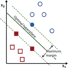
Figure 12.6 Optimal hyperplane and maximum margin [29].
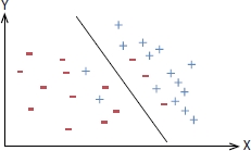
Figure 12.7 Support vector classifier.
![]() is the distance of the data point from the hyperplane, M is the margin, li = label,
is the distance of the data point from the hyperplane, M is the margin, li = label, ![]() = coefficients of the attributes, yi = data points of all attributes in each row, and ϵ is the slack variable. The left-hand side function in Equation (12.3) is the classification confidence and its value ≥ 1 shows that the classifier has identified the points correctly while value lesser than 1 shows that points are not being classified correctly hence a penalty of ϵi is incurred [30].
= coefficients of the attributes, yi = data points of all attributes in each row, and ϵ is the slack variable. The left-hand side function in Equation (12.3) is the classification confidence and its value ≥ 1 shows that the classifier has identified the points correctly while value lesser than 1 shows that points are not being classified correctly hence a penalty of ϵi is incurred [30].
12.2.7.3 Decision Tree
Decision tree is a supervised machine learning algorithm used for classification problems [31]. It uses a tree-like model to make predictions, and it resembles an upside-down tree. The objective of the decision tree is to split the data into multiple sets and then each set is further split into the subsets to make a decision.
Figure 12.8 shows a binary decision tree for a person is fit or not. It can be seen that the tree is split into sets, and again based on the questions, it is further split and this process continues till the final outcome is reached [31]. Every node will represent a test and those nodes which do not have descendants are called leaves. The decisions are lying at the leaves. For classification problem, every leaf will contain a class label.
A homogeneity measure (it gives measure how homogeneous a dataset is) is applied on a dataset and more homogeneous the dataset is, the less the variations among the labels for the different data points in the dataset and if the variations are more, the homogeneity will be less.
The objective of the decision tree algorithm is to generate partitions (by creating a test) in such a way which results in homogeneous data points with homogeneity as high as possible [32]. The working of decision tree is that one attribute is selected and data is split such that homogeneity increases after each split and it is continued till the resulting leaves are sufficiently homogeneous. The homogeneity is measured in terms of Gini Index, entropy, and information gain.
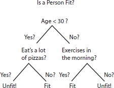
Figure 12.8 Binary decision tree [31].
Entropy quantifies the degree of disorder in the data, and its value varies from 0 to 1. If a data set is completely homogenous, then the entropy of such dataset is 0, i.e., there is no disorder. The entropy for a dataset D is defined as follows:
where Pi is the probability of finding a point with label i and k is the number of different labels.
ε[DA ] is the entropy of the partition after splitting on attribute A, ε[DA=i ] is the entropy of partition where the value of attribute A for the data points has value i, and DA=i is the number of data points for which value of attribute A is i and k is number of different labels.
Information gain [Gain (D,A)] measures reduction in entropy for the dataset D after splitting on the feature A, that is it is the difference between the original entropy ε[D ] and entropy obtained after partition on A ε[DA ].
12.2.7.4 Random Forest
Random forest is a popular supervised learning algorithm. It is a collection of decision trees and works on bagging technique which is an ensemble method [33]. In ensemble, instead of using an individual model, a collection of models is used to predict the output [34]. The most popular ensemble is the random forest which is a collection of many decision trees [7]. Bagging is the bootstrap aggregation where bootstrap refers to creating bootstrap samples for a given dataset containing 30% to 70% of the data and aggregation refers to aggregate the result of various models present in the ensemble [7]. It is a technique to select random samples from the dataset. Each of these samples is then used to train each tree in the forest.
The random forest is a classic ensemble technique which creates a collection of decision trees each of them built on different samples from the dataset, and it takes the majority score among these. A large number of trees as individual models ensures diversity that even if few trees overfit, the other trees in ensemble will take care of that and more diversity means the model is more stable. The independence among the trees results in a lower variance of the ensemble compared to a single tree which makes it computationally efficient. In this way, random forest controls the overfitting problem encountered with decision tree [13].
For a given dataset D with N attributes, each tree in the random forest can be created as: finding a bootstrap samples of D, then at each node selecting randomly a subset S from N attributes, evaluating the best split at each node from reduced subset of S features and growing the complete tree [7]. The total number of trees T and the attribute S at each node in the random forest are varied to have the best performance [7]. The error of the random forest is dependent on the correlation among the trees and the strength of the tree. If the correlation is less and strength high, then it results in low error. The low value of S implies low correlation and low strength between the trees, hence S is varied to obtain an optimal value [7]. The selection of features at each node is done majorly with Gini index. The outputs of each trees is then aggregated and the majority of the vote is used to predict the output case [7].
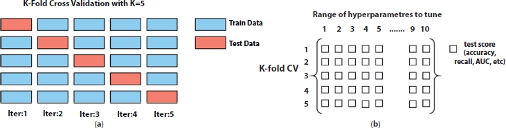
Figure 12.9 (a) Five-fold cross-validation technique and (b) GridSearchCV.
12.2.8 Tuning of Hyperparameters
Cross-validation technique is used to tune the values of hyperparameters. The data is first split into train and test, and then, the multiple models are trained by sampling the train set. In last, the test data is used to test the hyperparameter once. In this experiment, to avoid the overfitting problems, k-fold cross-validation technique with k = 5 is used to evaluate the fraud detection. Each time (for k = 5 here), k – 1 = 4 folds are used to build the model and the fifth fold is used to test the model. Figure 12.9a shows the five-fold cross-validation technique used for this experiment. The final result is then predicted from five trained models taking average from each subset and hence performance result gives accurate outputs.
As each machine learning algorithms have different hyperparameters, hence the search for finding the best model is completely different from each other. The technique used for tuning many hyperparameters at the same time is grid search cross validation, GridSearchCV, used in this experiment. The grid is a matrix (metrics such as accuracy and recall) which is populated on each iteration, as shown in Figure 12.9b.
12.2.9 Performance Evaluation of the Models
Different measures of classification performance are observed in Section 12.1. It is concluded that the overall accuracy is an insufficient performance measure for highly biased dataset because for all the transactions of majority class, even the default prediction will show a high performance [7]. The selected credit card dataset has only 0.172% fraud transactions with remaining as legitimate cases. It means even the classifier is not good enough, and then, also, it will give a high accuracy. Hence, other evaluation metrics like precision, recall, F1-score, and AUC should be investigated along with accuracy to check the performance of the models [7].
As the classification of transactions in two classes are being done, there are chances to incur some errors such as fraud cases being incorrectly classified as no-fraud and no-fraud cases being incorrectly classified as fraud cases. To capture these errors and to evaluate the performance of the model, confusion matrix is used which is shown in Table 12.2 [7].
Table 12.2 Confusion matrix [7].
| Predicted negative | Predicted positive | |
| Actual Negative | True Negative (TN) | False Positive (FP) |
| Actual Positive | False Negative (FN) | True Positive (TP) |
The confusion matrix shows four basic metrics: TP, TN, FP, and FN [7]. TP is the number of actual positive transactions predicted as positive; it means fraud cases are predicted as fraud. TN is the number of actual negative transactions predicted as negative; it means no-fraud transactions are predicted as genuine. FP is the number of actual negative transactions predicted as positive; it means no-fraud cases are predicted as fraud ones. FN is the number of actual positive transactions predicted as negative; it means fraud cases are predicted as no-fraud ones [35]. A good performance of fraud detection requires less number of FP and FN.
The performance of the logistic regression, SVM, decision tree, and random forest classifiers are evaluated based on accuracy, precision, recall, F1-score, MCC, AUC, and AUPRC [20].
The simplest model evaluation metric for classification models is accuracy which is the percentage of correctly predicted labels [7]. Recall (or sensitivity) tells the accuracy for fraud (positive) cases. Precision tells the accuracy on transactions predicted as fraud (positive) [35]. It is difficult to select the best model between different models with low recall and high precision or vice versa, in that case F1-score (or F-measure), which is the harmonic mean of precision and recall, is used [36].
MCC is a balanced performance measure used for a binary class problem and provides the good measure even when the dataset is unbalanced [37]. It is calculated using true and false negatives and positives.
A value of +1 for MCC shows the perfect prediction and a value of –1 shows the complete difference [37].
TPR tells the number of correctly predicted positive (fraud) cases divided by total number of positives cases which is same as recall (sensitivity) [38]. Whereas FPR tells the number of FPs (0s predicted as 1s) divided by total number of negatives [38]. On plotting TPR and FPR, a graph is found which shows the trade-off between the both and this curve is called ROC curve as shown in Figure 12.10a [38]. The area under the ROC curve is called AUC. For a good model, TPR should be high and FPR should be low and for this cut-off should be high.
The AUPRC is an important evaluation metrics for binary classification with highly imbalanced dataset [38]. Since the precision and recall are mainly concerned for the minority cases (here fraud cases) which makes the area under the precision and recall curve an important performance metrics for highly biased dataset [40]. It is the plot of recall and precision for various probability threshold as shown in Figure 12.10b. The area under the precision recall curve is investigated for evaluating the performance of the classifier [40, 41].
Once the optimum hyperparameters after tuning is obtained for each machine learning algorithm, the model is built with those hyperparameters using the train data. Then, this built model is used to evaluate the performance on the test data. In this experiment, the performance of the models is evaluated on the basis of recall, precision, accuracy, F1-score, MCC, AUC, and AUPRC. Since this work is mainly focused on the fraud detection of the credit card, hence the primary goal is that the models should detect all fraudulent transactions and for that “recall” score should be maximum; hence, it is used as “score” in the GridSearchCV for maximizing. Also at the same time, the precision should also not be very low else the genuine transaction will be predicted as fraud which can impact the customers. The F1-score, which is the harmonic mean of precision and recall, is also a good performance metric for this experiment. The best model is selected on the basis of good performance for all the above stated metrics.
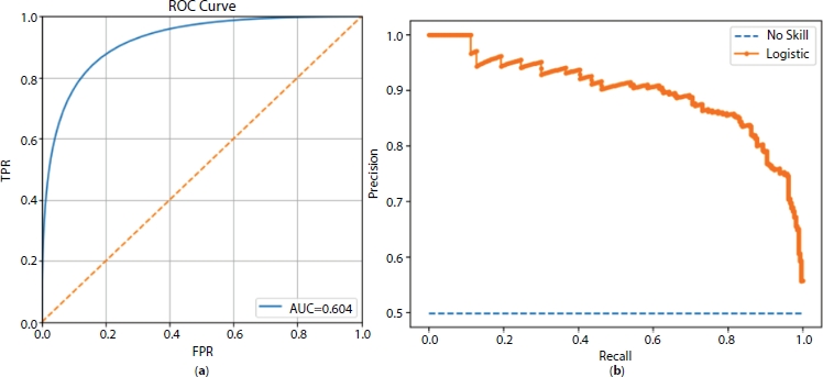
Figure 12.10 (a) ROC curve [39]. (b) Precision recall curve for no skill and logistic regression algorithms [40].
12.3 Results and Discussion
The results from the analysis and models implementation are discussed in this section. The outline of “Results and Discussion” is shown in Figure 12.11.
The cleaned and transformed data after EDA is modeled using different sampling techniques. The important thing to observe here for a better performance is that the transformed data needs to be split into train-test data before applying any balancing technique. It is done for holding the original test data for testing else the algorithms might use it (if not split) in the training phase and can lead to overfitting. As it can be noticed from Figure 12.11, the first implementation is done without using any of the sampling technique, to check the performance of the machine learning algorithms on the unsampled data.
Four different balancing techniques: RUS, ROS, SMOTE, and balanced class weight (class_weight = “balanced”) have been utilized to implement four machine learning techniques: logistic regression, decision tree, SVM, and random forest. The train dataset is modeled using the mentioned algorithms. The best hyperparameters of each model is searched using GridSearchCV of five-fold cross-validation technique. The built model (using the best hyperparameters) is used to predict the output for the test data, and then, the different performance metrics are calculated for fraud and genuine transactions. This method is followed for each of the built models.
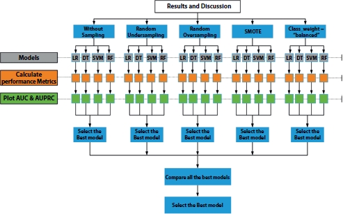
Figure 12.11 Outline of implementation and results.
12.3.1 Results Using Balancing Techniques
In RUS technique, the train dataset is random undersampled in which the majority class data (genuine ones) is reduced such that both the classes have same number of records. Here, the no-fraud transactions have been randomly reduced to the number of transactions equal to the fraud ones, both having same number of records of 344 in their train data.
For random oversampled technique, the train dataset is random oversampled in which the minority class data is increased such that both the classes have same number of records. Here, the fraud transactions have been randomly increased to the number of transactions equal to the no-fraud ones, both having same number of records of 199,020 in their train data.
For SMOTE technique, the minority class data is synthetically generated such that both the classes have same number of records. Here, the fraud transactions have been synthetically increased to the number of transactions equal to the no-fraud ones, both having same number of records of 199,020 in their train data.
The argument class_weight = “balanced” for balanced class weight is used for class imbalance problem. It penalizes the errors on the class having lower number of records by the same amount. It is used for all the four algorithms to check if any better performance value is obtained without using the sampling technique.
After using the balancing techniques, the implementations are done again using all the four machine learning algorithms for each of them.
12.3.2 Result Summary
The results for the implemented models have been collated here. In this experiment, total of 20 models have been implemented using permutation and combination of different balancing techniques with four machine learning algorithms. Table 12.3 summarizes the results for all the implemented models.
Table 12.3 Result summary for all the implemented models.
| Algorithm | Sampling technique | Accuracy | Precision | Recall | Fl-score | MCC | ROC | AUPRC |
|
Logistic Regression | Without sampling | 99.92% | 86.11% | 62.84% | 72.66% | 0.74 | 0.95 | 0.71 |
| RUS | 97.43% | 5.64% | 87.84% | 10.59% | 0.22 | 0.97 | 0.66 | |
| ROS | 97.84% | 6.65% | 87.84% | 12.36% | 0.24 | 0.968 | 0.73 | |
| SMOTE | 97.78% | 6.46% | 87.84% | 12.04% | 0.23 | 0.965 | 0.74 | |
| Balanced class weight | 98.08% | 7.33% | 86.49% | 13.52% | 0.25 | 0.97 | 0.69 | |
| Decision Tree | Without sampling | 99.93% | 76.58% | 81.76% | 79.08% | 0.79 | 0.935 | 0.74 |
| RUS | 92.96% | 2.20% | 91.22% | 4.29% | 0.14 | 0.948 | 0.45 | |
| ROS | 99.15% | 13.77% | 74.32% | 23.23% | 0.32 | 0.87 | 0.7 | |
| SMOTE | 97.46% | 5.19% | 79.05% | 9.74% | 0.2 | 0.89 | 0.65 | |
| Balanced class weight | 95.03% | 2.96% | 87.16% | 5.72% | 0.16 | 0.93 | 0.66 | |
| SVM | Without sampling | 99.92% | 78.47% | 76.35% | 77.40% | 0.77 | 0.927 | 0.71 |
| RUS | 96.77% | 4.53% | 87.84% | 8.61% | 0.2 | 0.969 | 0.67 | |
| ROS | 99.75% | 37.21% | 64.86% | 47.29% | 0.49 | 0.86 | 0.44 | |
| SMOTE | 99.64% | 27.17% | 65.54% | 38.42% | 0.42 | 0.957 | 0.44 | |
| Balanced class weight | 99.67% | 29.34% | 66.22% | 40.66% | 0.44 | 0.97 | 0.38 | |
| Random Forest | Without sampling | 99.94% | 92.37% | 73.65% | 81.95% | 0.82 | 0.927 | 0.81 |
| RUS | 97.49% | 5.68% | 86.49% | 10.65% | 0.22 | 0.967 | 0.69 | |
| ROS | 99.94% | 87.02% | 77.03% | 81.72% | 0.82 | 0.93 | 0.82 | |
| SMOTE | 99.92% | 76.43% | 81.08% | 78.69% | 0.79 | 0.96 | 0.81 | |
| Balanced class weight | 99.95% | 97.27% | 72.30% | 82.95% | 0.84 | 0.92 | 0.82 |
The intention of any credit card fraud detection is to identify the fraud cases correctly, i.e., to have a better value of the recall of the fraudulent transaction. Also, the fraudulent transaction dominates the credit card fraud detection; hence, a high recall value (accuracy on fraud cases) instead of overall accuracy is the requirement. As seen from the results in Table 12.3, all the machine learning algorithms without using any sampling technique have shown a low recall value and a high precision value. The research objective of this study is to obtain a suitable balancing technique to be applied on the highly skewed dataset for getting better performance of the models. Table 12.3 shows that all the models with RUS technique have resulted in a good recall but at the cost of very low precision and a low F1-score with low MCC and a low AUPRC value. The recall is increased using the ROS technique but even though the precision and F1-score with MCC and AUPRC are not in a good range. Only random forest model has performed well with ROS technique, whereas all other models have shown not so good results. SMOTE oversampling has performed well with the models and it has increased the recall for random forest resulting in better performance metrics compared to the other models. One important thing to notice here is that, without using any sampling technique for all the models and using the “balanced” class weight configuration for the machine learning algorithms, a good result (except low precision) is achieved for all the classifiers. Hence, it can be inferred that SMOTE oversampling technique has provided a good result.
This work has started with a motive to get the better result for all the selected performance metrics: recall, precision, accuracy, F1-score, MCC, AUC, and AUPRC. On comparing the results in Table 12.3, it can be observed that the highest recall of 91.22% is obtained for the decision tree model with RUS technique. But this model has a precision of only 2.20%, F1-score of 4.29%, MCC of 0.14, and AUPRC of 0.45; hence, this cannot be considered as the best model. It can also be noticed from Table 12.3 that the random forest even without using any sampling technique has done well in terms of all the performance metrics compared to the other machine learning algorithms. It shows the strength of the ensemble model even with the imbalanced dataset. Also, the result for random forest with SMOTE technique is around the same using the “balanced” class weight configuration with recall value lower than SMOTE. As expected, the accuracy and AUC are not the accurate measures for the credit card fraud detection as it has approximately same values (greater than 90%) for all the implemented models.
As seen in other literatures, there is no fixed performance metrics for the fraud detection as it depends on the business requirement. But, what is important for the credit card fraud detection is that, if a fraud transaction is misclassified as a genuine one, it will definitely cause severe problems. At the same time, no one will want to misclassify a genuine transaction as a fraud one. Hence, a good performance of the fraud detection should have lesser number of FN and FP. Table 12.4 collates the result of confusion matrix of all the implemented models. It can be seen that the lowest value of FN, FN is 13 for decision tree model with RUS technique, but it has a high FP, FP cases with a value of 6,006 which is unacceptable. The random forest model with SMOTE oversampling has a less number of FN cases: 28 with less number of FP cases: 37 compared to the other models. It can also be noticed that the random forest model with class_weight = “balanced” has the lowest FP with a value of 3 and a lower FN cases as 41.
Comparing the results from Tables 12.3 and 12.4 for each of the machine learning algorithms, it can be deduced that the logistic regression model has given the best recall with SMOTE oversampling technique but not good values for other parameters. This model has shown lower FN cases of value 18 but higher FP cases as 1,881. The decision tree classifier has performed well with RUS technique giving the maximum recall obtained in this experiment but at lower values for all other performance metrics. Also, it has output in a high FP cases with value of 6,006 with low FN cases value of 13. SVM with RUS has given a good recall with a lower performance values for other parameters. This model has shown a low number of FN cases as 18 but with a higher FP cases with value of 2741. The random forest has performed great with SMOTE oversampling and balanced class weight technique both.
This work is focused on obtaining a model with good values for all the performance metrics rather than improving any one parameter and with a less number of FN and FP at the same time. Hence, the best model should not only give a high recall value, but a good value of precision, good accuracy, better F1-score, good MCC, high values of AUC and AUPRC. Comparing all the results from Tables 12.3 and 12.4, it can be seen that the random forest with balanced class weight has demonstrated a good result with the highest precision of 97.27%, the highest F1-score of 82.95% and the highest MCC value of 0.84 compared to all other models with AUC value of 0.92 and AUPRC of 0.82. But this model has shown a lower recall of 72.30%. Hence, it is concluded that the Random forest with SMOTE oversampling technique has provided the best result in terms of all the mentioned performance metrics with accuracy of 99.92%, recall value of 81.08%, precision of 76.43%, F1-score of 78.69%, MCC of 0.79, AUC of 0.96, and AUPRC as 0.81. It also has output the less number of FN transactions with value as 28 and less number of FPs with value as 37. Using the best model of this random forest for SMOTE oversampled data, the features are ranked in order of importance and it is observed that feature V14 is the most important variable selected by this model followed by V10, V17, V11, and V4.
Table 12.4 Confusion matrix results for all the implemented models.
| Algorithm | Sampling technique | TN (No-Fraud) | FP | FN | TP (Fraud) |
|
Logistic Regression | Without sampling | 85,280 | 15 | 55 | 93 |
| RUS | 83,119 | 2,176 | 18 | 130 | |
| ROS | 83,470 | 1,825 | 18 | 130 | |
| SMOTE | 83,414 | 1,881 | 18 | 130 | |
| Balanced class weight | 83,677 | 1,618 | 20 | 128 | |
|
Decision Tree | Without sampling | 85,258 | 37 | 27 | 121 |
| RUS | 79,289 | 6,006 | 13 | 135 | |
| ROS | 84,606 | 689 | 38 | 110 | |
| SMOTE | 83,157 | 2,138 | 31 | 117 | |
| Balanced class weight | 81,064 | 4,231 | 19 | 129 | |
| SVM | Without sampling | 85,264 | 31 | 35 | 113 |
| RUS | 82,554 | 2,741 | 18 | 130 | |
| ROS | 85,133 | 162 | 52 | 96 | |
| SMOTE | 85,035 | 260 | 51 | 97 | |
| Balanced class weight | 85,059 | 236 | 50 | 98 | |
|
Random Forest | Without sampling | 85,286 | 9 | 39 | 109 |
| RUS | 83,168 | 2,127 | 20 | 128 | |
| ROS | 85,278 | 17 | 34 | 114 | |
| SMOTE | 85,258 | 37 | 28 | 120 | |
| Balanced class weight | 85,292 | 3 | 41 | 107 |
12.4 Conclusions
This paper researched how the balancing techniques along with different machine learning algorithms can be utilized to account the problem of credit card fraud detection and to obtain a better result. In particular, this work has tried to get a better performance for the model in terms of all the mentioned metrics rather than anyone of them. The random forest with SMOTE oversampling has provided the best result in terms of all the selected performance metrics with accuracy of 99.92%, recall value of 81.08%, precision of 76.43%, F1-score of 78.69%, MCC of 0.79, AUC of 0.96, and AUPRC of 0.81. It also has resulted in less number of FN transactions with value as 28 and less number of FPs with value as 37. The key point of this study is that, unlike other reported works, the balancing technique to handle the highly biased dataset is not fixed before implementing the model and all the balancing methods are implemented with all the classifiers to select the best one. In addition to the sampling techniques, this work has also used the balanced class weight at the modeling time for all the algorithms for considering the biased nature of the dataset. The contribution of this thesis toward credit card fraud detection is achieving a comparable result considering the balanced class weight and without using any sampling technique. The other major point that distinguishes this study from others is that this work is not only focused on the mentioned machine learning algorithms, rather than the permutation and combination of these methods with several result parameters and with different balancing techniques are studied and analyzed for several evaluation metrics to obtain a better outcome. As a result, total of 20 models have been implemented, compared and analyzed to get the best output.
12.4.1 Future Recommendations
In future, a cost-sensitive learning technique can be carried out on this study by evaluating the misclassification costs. The misclassification cost for a fraudulent transaction as a genuine one (FN) known as the fraud amount is higher than the misclassification cost for a genuine case as a fraudulent case (FP), and it is related to the cost for contacting and analyzing the customer. The machine learning techniques can be implemented considering these different costs of misclassifications and to evaluate the performance metrics. The algorithmic ensemble techniques can be used to balance the dataset and to evaluate the performance of the models implemented for this work. An ensemble technique combining the random forest (best model of this study) with neural networks can be implemented as a future work. As there is continuous evolution to avoid the fraud detection by the fraudsters, hence the non-stationary behavior of credit card fraud can be considered for the model building. Also, the hybrid approach of undersampling and oversampling technique along with other sampling techniques can be investigated as a future work.
References
1. Landes, H., Credit Card Basics: Everything You Should Know, Forbes, USA, 2013, [Online]. Available: https://www.forbes.com/sites/moneybuilder/2013/06/11/credit-card-basics-everything-you-should-know/#5f26b45d42c0.
2. Rajora, S. et al., A comparative study of machine learning techniques for credit card fraud detection based on time variance. Proc. 2018 IEEE Symp. Ser. Comput. Intell. SSCI 2018, March 2019, pp. 1958–1963, 2019.
3. Rohilla, A. and Bansal, I., Credit Card Frauds : An Indian Perspective. Adv. Econ. Bus. Manage., 2, 6, 591–597, 2015.
4. Seeja, K. R. and Zareapoor, M., FraudMiner: A novel credit card fraud detection model based on frequent itemset mining. Sci. World J., 2014, 252797, 10, 2014. https://doi.org/10.1155/2014/252797.
5. Awoyemi, J.O., Adetunmbi, A.O., Oluwadare, S.A., Credit card fraud detection using machine learning techniques: A comparative analysis. Proc. IEEE Int. Conf. Comput. Netw. Informatics, ICCNI 2017, Janua, vol. 2017, pp. 1–9, 2017.
6. Seeja, K.R. and Zareapoor, M., FraudMiner: A novel credit card fraud detection model based on frequent itemset mining. Sci. World J., 2014, 3–4, 2014.
7. Bhattacharyya, S., Jha, S., Tharakunnel, K., Westland, J.C., Data mining for credit card fraud: A comparative study. Decis. Support Syst., 50, 3, 602–613, 2011.
8. Dal Pozzolo, A., Caelen, O., Le Borgne, Y.A., Waterschoot, S., Bontempi, G., Learned lessons in credit card fraud detection from a practitioner perspective. Expert Syst. Appl., 41, 10, 4915–4928, 2014.
9. Sohony, I., Pratap, R., Nambiar, U., Ensemble learning for credit card fraud detection. ACM Int. Conf. Proceeding Ser., pp. 289–294, 2018.
10. Sorournejad, S., Zojaji, Z., Atani, R.E., Monadjemi, A.H., A survey of credit card fraud detection techniques: Data and technique oriented perspective. 1–26, 2016. arXiv:1611.06439 [cs.CR].
11. Carcillo, F., Dal Pozzolo, A., Le Borgne, Y.A., Caelen, O., Mazzer, Y., Bontempi, G., SCARFF: A scalable framework for streaming credit card fraud detection with spark. Inf. Fusion, 41, 182–194, 2018.
12. Dal Pozzolo, A., Boracchi, G., Caelen, O., Alippi, C., Bontempi, G., Credit card fraud detection: A realistic modeling and a novel learning strategy. IEEE Trans. Neural Networks Learn. Syst., 29, 8, 3784–3797, 2018.
13. Navanshu, K. and Saad, Y.S., Credit Card Fraud Detection Using Machine Learning Models and Collating Machine Learning Models. J. Telecommun. Electron. Comput. Eng., 118, 20, 825–838, 2018.
14. Mekterović, I., Brkić, L., Baranović, M., A systematic review of data mining approaches to credit card fraud detection. WSEAS Trans. Bus. Econ., 15, 437–444, 2018.
15. Puh, M. and Brkić, L., Detecting credit card fraud using selected machine learning algorithms. 2019 42nd Int. Conv. Inf. Commun. Technol. Electron. Microelectron. MIPRO 2019 - Proc., pp. 1250–1255, 2019.
16. Kumar, A. and Garima, G., Fraud Detection in Online Transactions Using Supervised Learning Techniques, in: Towards Extensible and Adaptable Methods in Computing, pp. 309–386, Springer, Canada,2018.
17. Mittal, S. and Tyagi, S., Performance evaluation of machine learning algorithms for credit card fraud detection. Proc. 9th Int. Conf. Cloud Comput. Data Sci. Eng. Conflu. 2019, pp. 320–324, 2019.
18. Yee, O.S., Sagadevan, S., Malim, N.H.A.H., Credit card fraud detection using machine learning as data mining technique. J. Telecommun. Electron. Comput. Eng., 10, 1–4, 23–27, 2018.
19. Dal Pozzolo, A., Adaptive Machine Learning for Credit Card Fraud Detection Declaration of Authorship, PhD Thesis, p. 199, December 2015.
20. Kaggle, 2018. [Online]. Available: https://www.kaggle.com/mlg-ulb/credit-cardfraud/data#creditcard.csv.
21. Wen, S.W. and Yusuf, R.M., Predicting Credit Card Fraud on a Imbalanced Data. Int. J. Data Sci. Adv. Anal. Predict., 1, 1, 12–17, 2019.
22. Collell, G., Prelec, D., Patil, K.R., A simple plug-in bagging ensemble based on threshold-moving for classifying binary and multiclass imbalanced data. Neurocomputing, 275, 330–340, 2018.
23. Estabrooks, A., Jo, T., Japkowicz, N., A multiple resampling method for learning from imbalanced data sets. Comput. Intell., 20, 1, 18–36, 2004.
24. Chawla, N.V., Bowyer, K.W., Hall, L.O., SMOTE: Synthetic Minority Oversampling Technique. J. Artif. Intell. Res., 16, 1, 321–357, 2002.
25. Tara, B., Dealing with Imbalanced Data, towards data science, 2019, [Online]. Available: https://towardsdatascience.com/methods-for-dealing-with-imbalanced-data-5b761be45a18.
26. AnalyticsVidhya, Imbalanced Data : How to handle Imbalanced Classification Problems, Analytics Vidhya, Indore, 2017, [Online]. Available: https://www.analyticsvidhya.com/blog/2017/03/imbalanced-data-classification/.
27. elitedatascience, How to Handle Imbalanced Classes in Machine Learning, elitedatascience, 2019, [Online]. Available: https://elitedatascience.com/imbalanced-classes.
28. Ayush, P., Introduction to Logistic Regression, towards data science, 2019, [Online]. Available: https://towardsdatascience.com/introduction-to-logistic-regression-66248243c148.
29. Rohith, G., Support Vector Machine — Introduction to Machine Learning Algorithms, towards data science, 2018, [Online]. Available: https://towards-datascience.com/support-vector-machine-introduction-to-machine-learning-algorithms-934a444fca47.
30. Misra, R., Support Vector Machines — Soft Margin Formulation and Kernel Trick, towardsdatascience, 2019, https://towardsdatascience.com/, [Online]. Available: https://towardsdatascience.com/support-vector-machines-soft-margin-formulation-and-kernel-trick-4c9729dc8efe#:~:text=how they work.-, Soft Margin Formulation, modifying the objective of SVM.
31. Mayur, K., Decision Trees for Classification: A Machine Learning Algorithm, Xoriant, 2017, [Online]. Available: https://www.xoriant.com/blog/product-engineering/decision-trees-machine-learning-algorithm.html.
32. Prince, Y., Decision Tree in Machine Learning, towards data science, 2018, [Online]. Available: https://towardsdatascience.com/decision-tree-in-machine-learning-e380942a4c96.
33. tutorialspoint, Classification Algorithms - Random Forest, tutorialspoint, 2019, [Online]. Available: https://www.tutorialspoint.com/machine_learning_with_python/machine_learning_with_python_classification_algorithms_random_forest.htm.
34. Tony, Y., Understanding Random Forest, towards data science, 2019, [Online]. Available: https://towardsdatascience.com/understanding-random-forest-58381e0602d2.
35. Awoyemi, J.O., Adetunmbi, A.O., Oluwadare, S.A., Credit card fraud detection using machine learning techniques: A comparative analysis. Proc. IEEE Int. Conf. Comput. Netw. Informatics, ICCNI 2017, Janua, vol. 2017, pp. 1–9, 2017.
36. Prabhu, Understanding Hyperparameters and its Optimisation techniques, towardsdatascience, 2018, [Online]. Available: https://towardsdatascience.com/understanding-hyperparameters-and-its-optimisation-techniques-f0debba07568#:~:text=What are Hyperparameters%3F, Model parameters vs Hyperparameters.
37. Randhawa, K., Loo, C.K., Seera, M., Lim, C.P., Nandi, A.K., Credit Card Fraud Detection Using AdaBoost and Majority Voting. IEEE Access, 6, 14277–14284, 2018.
38. Jason, B., How to Use ROC Curves and Precision-Recall Curves for Classification in Python, Machine Learning Mastery, 2018, [Online]. Available: https://machinelearningmastery.com/roc-curves-and-precision-recall-curves-for-classification-in-python/.
39. Nazrul, S.S., Receiver Operating Characteristic Curves Demystified (in Python), towards data science, 2018, [Online]. Available: https://towards-datascience.com/receiver-operating-characteristic-curves-demystified-in-python-bd531a4364d0.
40. Brownlee, J., ROC Curves and Precision-Recall Curves for Imbalanced Classification, Machine Learning Mastery, 2020, [Online]. Available: https://machinelearningmas-tery.com/roc-curves-and-precision-recall-curves-for-imbalanced-classification/.
41. Asare-Frempong, J. and Jayabalan, M., Predicting customer response to bank direct telemarketing campaign. 2017 Int. Conf. Eng. Technol. Technopreneurship, ICE2T 2017, January, vol. 2017, pp. 1–4, 2017.
- Email: [email protected]