
8
Machine Learning and Deep Learning for Medical Analysis—A Case Study on Heart Disease Data
Swetha A.M., Santhi B.* and Brindha G.R.
SASTRA Deemed University, Thanjavur, Tamil Nadu, India
Abstract
Cardiovascular diseases (CVDs) encompass a variety of heart problems ranging from vascular disorders like coronary heart diseases and peripheral arterial disorders to morbid cardiac diseases like heart failure (or myocardial infarction) and cardiomyopathy, to name a few. These diseases often occur as repercussions of low cardiac output and decreased ejection factor, usually exacerbated by vascular blockages. With the increasing severity of CVDs, a need for predicting heart failures is on the rise, but the traditional methods employed for CVD-related event prediction, unfortunately, have failed to achieve the acme of accuracy. Given a set of medical records as datasets, Machine Learning (ML) can be employed to achieve high accuracy in the prediction of patient survival and also in determining the driving factors that increase mortality among CVD patients. The medical records that provide the necessary data for prediction form a basic framework that divulges inconspicuous consistencies of patient’s data which along with an appropriate ML algorithm confute the traditional methods thereby providing a strong base for determining the feature that contributes the most for the risk factor. The proposed model uses various feature selection techniques to extract those features in particular that highly contributes to the prediction of the target attribute and exploits the application of ML and Deep neural classifier algorithms to predict possibilities of CVD development among patients. Our results show that follow-up time, ejection fraction, and serum creatinine as the most significant features that affect the survival rate of the heart failure patient when compared to other features giving an accuracy of 99.1% using XGBoost.
Keywords: Cardiovascular diseases, heart failure, ejection fraction, serum creatinine, feature selection
8.1 Introduction
Cardiovascular diseases (CVDs) [25] have become more prevalent in recent times with mortality rates counting as high as 15–17 million per year, which is about 30%–31% of the total deaths worldwide according to the WHO reports. Myocardial infarction, coronary heart diseases, and arrhythmia are some of the most common CVDs. The precarity of CVD makes it one of the most treacherous diseases that prevail presently in society. What accounts for this unpredictability is the diversity of contributing features that range from inevitable factors like inheritance, age, gender to avoidable ones like alcohol abuse and tobacco consumption. Recent medical reports reveal that about 80% of the patients who die premature (below the age of 70) fall under the elderly category and about 25% of the remaining are middle-aged women. Though these factors (age and sex of the patient) are not the best way to discern the worst of the cases, they cannot be entirely disregarded. Other clinical factors like the concentration of serum creatinine and ejection fraction play more prominent roles in patients’ survival prediction, especially for those that have been receiving treatment over a period of time.
Considering the diversity of causal factors associated with CVDs, it remains a challenge to sort out the significant features that may aid in timely prediction of a patient’s survival. Filtering the prominent factors requires careful perusal through different medical records to note the degree of influence a specific factor exerts on the patient’s survival.
Hence, to ensure high efficacy and maximum accuracy, Machine Learning (ML) models could be exploited, as have been in the proposed model. ML models can be used for meticulous prediction of the target variable (which in this case is the survival rate of a patient) by taking into account several affecting features. The affecting features, however, could be a mix of both important as well as less-influential factors. Hence, to overcome this challenge, the proposed model employs feature selection methods.
The dataset used to train and test the ML models was obtained from live medical records [22] collected at the Faisalabad Institute of Cardiology and at the Allied Hospital in Faisalabad (Pakistan) from April to December 2015. The dataset contains the records of 299 heart failure patients, about 105 of which are women and whose age ranges from 40 to 95 years. All the patients listed in the records had suffered left ventricular dysfunction and had a history of cardiac arrests and fall under class III and IV of heart failure stages as deemed by New York Heart Association (NYHA) [7].
The dataset, which entails these live medical records, is normalized to treat outliers and other noise that may interfere with the model’s predictive potential and also oversampled as the data showed conspicuous imbalance between classes.
Feature selection methods, like Extra Tree Classifiers, Pearson Correlation, Forward Selection, and Chi-square tests, were performed to sort out the most prominent features. Serum creatinine concentration, ejection fraction, age of the patients, and the duration of treatment were proved to have maximum influence on the patients’ death event and were hence used as cardinal predictive variables in the model. Doing this increased the model’s prediction accuracy to about 75%.
The proposed model constitutes several ML algorithms like SVM, CNN [26], and other ensemble methods that are trained on the set of medical records. These algorithms were weighed individually based on their accuracy score for different sets of features. The models were trained over three different studies: one with follow-up time, creatinine level, and ejection fraction as major factors, another with age instead of follow-up time and the third over the entire set of features available in the dataset.
8.2 Related Works
Chronic cardiac failure occurs when the fluid accumulates around the heart, causing it to pump insufficiently for the body to function normally. There are two types of chronic cardiac failure based on left ventricular function: systolic heart failure (reduced ejection fraction HFrEF) and diastolic heart failure. For normal people, the percentage of blood that is pumped out by the left ventricle in each contraction is 50%–70%. The reduced ejection fraction [18] is a case which occurs if the ejection fraction is below 40% without much effective contraction by the heart muscles. The causes of HFrEF are Ischemic cardiomyopathy and dilated cardiomyopathy. The diastolic heart failure [19] occurs when there is a normal contraction in heart muscles but no relaxation in ventricles during ventricular filling. With the increasing severity of CVDs, a need for predicting heart failures is on the rise but the traditional methods employed for CVD-related event prediction, unfortunately have failed to achieve the acme of accuracy.
Given a set of medical records as datasets, ML can be employed to achieve high accuracy in the prediction of patient survival and also in determining the driving factors like ejection fraction and serum creatinine [8] that increase mortality among CVD patients.
According to the NYHA, the heart failure is classified into four classes [5] based on the heart failure symptoms. Class I is where the patient experiences asymptomatic left ventricular dysfunction with normal physical activities, Class II with slight symptoms and limited physical activities, Class III with modest symptoms and very few physical activities, and Class IV with severe symptoms on complete rest. The dataset used in this analysis consists of 299 patients with left ventricular dysfunction belonging to Class III or IV [7].
The survival rate and the heart failure hospitalizations of patients suffering from heart failure due to preserved ejection fraction [6] using various ML models like logistic regression, SVM, random forest, and gradient descent boosting are predicted. Lasso regression and forward selection feature selection techniques [4] were used to find that blood urea nitrogen levels, cardiomyopathy questionnaire subscore, and body mass index are the most significant features affecting the survival rate of the patients. The random forest is found to be the best model for predicting the survival rate of the HFpEF patient with an AUC of 0.76.
The decision tree boosting model is trained using 5822 records of the patients in the UCSD Cohort [1, 9] with eight clinical features: diastolic blood pressure, creatinine, blood urea nitrogen, hemoglobin, white blood cell count, platelets, albumin, and red blood cell distribution width. The decision tree is the best classifier with AUC of 0.88. The Cox regression model [2] predicts that age is the most significant feature that affects the survival rate of the patient and with an increase in each year the mortality rate increases by 4%. The next most significant features are ejection fraction and serum creatinine with a p-value of 0.0026, and it is evident that the rate of survival decreases doubly with a one-unit increase in serum creatinine. Serum sodium and anemia were also significant with a p-value of 0.0052 and 0.0096, respectively. Other features like gender, smoking creatinine phosphokinase, and platelets were not significant for predicting the survival rate as these parameters may be significant at the initial stage of heart failure but this analysis contains patients at stage III or IV of heart failure.
The preceding studies presents finding the significant features using statistical methods, which leaves a plenty of space for various ML-based feature selection methods in healthcare services. The aim of this study is to address the issue of efficiency using various feature selection methods to rank the importance of the features in predicting the survival rate. Figure 8.1 shows the workflow model of the proposed methodology.
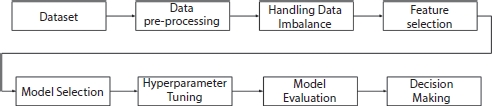
Figure 8.1 Workflow model of proposed system.
8.3 Data Pre-Processing
Data pre-processing [3] is a cardinal method in data mining technique as it involves cleaning and organizing the data before being used. Processing of data is crucial as it may contain undesirable information such as outliers, noise, duplicate data, and, sometimes, even wrong data which might be misleading. In order to service these complications, data needs to be processed prior to its utilization. Sometimes, data may contain non-numeric and null values or missing attribute values along with imbalanced data. These issues can also be resolved using data pre-processing techniques. The most common procedures involved are data normalization, data wrangling, data resampling, and binning.
8.3.1 Data Imbalance
The distribution of data equally among the classes in the classification problem is one of the most important issues to be addressed to avoid misclassification due to severely skewed classes. There are various techniques to encounter class imbalance problems in the dataset. One of the techniques used for this analysis is Synthetic Minority Oversampling TEchnique (SMOTE).
SMOTE [27] is an oversampling method which is used to scale up the minority class in the dataset. A minority class is a class that is under-sampled or in other words has significantly less data samples that fall under it. The presence of such imbalance may cause the training model to often overlook the minority classes; since training models have the propensity to consider the majority classes due to the considerable amount of training data they happen to possess. SMOTE is one of the techniques used to resample the minority classes to achieve equal proportions of data samples as is distributed among other classes. In SMOTE, the oversampling (or resampling) is achieved by considering all the data points that fall under the minority class and connecting each point to its k-nearest homologous neighbors. After repeating this for all the data points, the model artificially synthesizes or creates sample points that lie on the lines joining the original data points. The resampling is done until the data becomes balanced. ADAptive SYNthetic (ADASYN) imbalance learning technique is similar to SMOTE when it comes to the initial oversampling procedures. The data points are connected to each of their k-nearest neighbors and sample points are created on those connecting lines. But in ADASYN, the points are instead placed closer to those lines as opposed to on them, thereby inducing variation in the data samples.
8.4 Feature Selection
Feature selection or variable selection is a cardinal process in the feature engineering technique [14] which is used to reduce the number of dependent variables by picking out only those that have a paramount effect on the target attribute (survival rate in this case). By employing this method, the exhaustive dataset can be reduced in size by pruning away the redundant features [17] that reduces the accuracy of the model. Doing this will help curtail the computational expense of modeling and, in some cases, may also boost the accuracy of the implemented model [13].
The feature selection models applied herein to achieve maximum accuracy in target prediction encompass the following:
- 1) Extra Tree Classifier
- 2) Pearson Correlation
- 3) Forward selection
- 4) Chi-square
- 5) Logit (logistic regression model)
The features that recurred in at least three of the above-mentioned models were assumed as having maximum impact on the target variable and were accordingly classified to fit into the employed ML model.
8.4.1 Extra Tree Classifier
The Extra Tree Classifier or the Extremely Random Tree Classifier [21] is an ensemble algorithm that seeds multiple tree models constructed randomly from the training dataset and sorts out the features that have been most voted for. It fits each decision tree on the whole dataset rather than a bootstrap replica and picks out a split point at random to split the nodes. The splitting of nodes occurring at every level of the constituent decision trees are based on the measure of randomness or entropy in the sub-nodes. The nodes are split on all variables available in the dataset and the split that results in the most homogenous sub-childs is selected in the constituent tree models. But unlike other tree-based ensemble algorithms like random forest, an Extra Tree Classifier does not choose the split that results in most homogeneity; instead, it picks a split randomly from the underlying decision tree framework. This lowers the variance and makes the model less prone to overfitting.
8.4.2 Pearson Correlation
Pearson Correlation is used to construct a correlation matrix that measures the linear association between two features and gives a value between –1 and 1, indicating how related the two features are to one another. Correlation is a statistical metric for measuring to what degree two features are interdependent and by computing the association between each feature and the target variable, the one exerting high impact on the target can be picked out. In other words, this model helps determine how a change in one variable reflects on the outcome. The measure of linear association between the features is given by the Pearson Correlation Coefficient which can be computed using the equation:
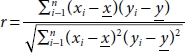
where xi is the ith value of the variable x, ![]() is the average value of sample attribute x, n is the number of records in the dataset, and x and y are the independent and target variables. A value of 1 indicates positive correlation, –1 indicates negative correlation, and 0 indicates no correlation between the features.
is the average value of sample attribute x, n is the number of records in the dataset, and x and y are the independent and target variables. A value of 1 indicates positive correlation, –1 indicates negative correlation, and 0 indicates no correlation between the features.
8.4.3 Forward Stepwise Selection
Forward selection is a wrapper model that evaluates the predictive power of the features jointly and returns a set of features that performs the best. It adds predictors to the model one at a time and selects the best model for every combination of features based on the cumulative residual sum of squares. The model starts basically with a null value and with each where xi is the ith value of the variable x, iteration the best of the attributes are chosen and added to the reduced list. The addition of features continues so far as the incoming variable has no impact on the model’s prediction and if such a variable is encountered it is simply ignored.
8.4.4 Chi-Square Test
A chi-square test is used in statistical models to check the independence of attributes. The model measures the degree of deviation between the expected and actual response. Lower the value of Chi-square, less dependent the variables are to one another and higher the value more is their correlation. Initially the attributes are assumed to be independent which forms the null hypothesis. The value of the expected outcome is computed using the following formula:
Chi-square is obtained from the expression that goes as follows:
where i is in the range (1, n), n is the number of dataset records, Oi is the actual outcome, and Ei is the expected outcome.
8.5 ML Classifiers Techniques
Classification models predict the classes or categories of given features using a variety of ML models. The classification algorithms can be classified into different models.

8.5.1 Supervised Machine Learning Models
Supervised learning is a branch of ML wherein a model is trained on a labeled dataset to deduce a learning algorithm. This is achieved by allowing the model to make random predictions and to correct and teach itself using the labels available. This happens iteratively until the learning algorithm specific to the data has been deduced and the model has achieved considerable accuracy. Supervised learning is a powerful technique in training ML models and is predominantly used. It can be classified into regression and classification based on whether the data is continuous or categorical.
8.5.1.1 Logistic Regression
As opposed to its name, a logistic regression model is a binary classifi-cation algorithm used when the target variable is categorical, or in other words when the target variable could be grouped into two different classes. The prediction is done by fitting the data to an activation function (a sigmoid logistic function) which returns a value between 0 and 1. The returned value determines how strongly a data entry belongs to one of the binary classes. This approach not only helps achieve higher accuracy but also ensures great precision, which makes it an ubiquitous, fundamental, and handy algorithm for binary classification. This statistical model can be mathematically formulated as follows:
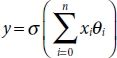
where σ is the logistic function applied to a weighted sum of independent variables xi: i ∈ (0, n), where n is the total number of data entries available in the dataset. Conventionally, x0 is assigned the value of 1 which leaves just θ0 in the sum, which is considered as a bias. A bias term is included so that even when the model is applied over no independent variable or the sum merely cancels all the terms (positive and negative) the final result does not come to be 0. This makes sense because σ(0) returns 0.5 which is ambiguous since class prediction becomes vague at that point.
8.5.1.2 SVM
Support Vector Machines (SVM) is a classification algorithm that introduces a best suited decision boundary which splits the dataset accordingly. It is generally used for binary classification but can also be extended to multi-class classification. SVM relies on Support Vectors, which are the data points that are closest to the hyperplane used to classify the data-set. For datasets that cannot be split using a decision boundary, an SVM model uses kernels to extend the data points to a higher dimension and by constructing a hyperplane to separate the classes. The kernels used are of two types: polynomial and radial. SVM models have higher accuracy even when fit to smaller data samples and in some cases may also outperform neural networks.
8.5.1.3 Naive Bayes
Naive Bayes is a fast learning classification algorithm based on Bayes’ theorem. The reason it is called naive is because the algorithm supposes the independence of the predictor variables. Or in other words, it assumes that a particular feature is not affected by the presence of other features. For each data point, the algorithm predicts the probability of how related the feature is to that class and the class for which the probability ranks highest is chosen as a probable class [23].
Bayes’ theorem can be given as follows:
where P(c|xi) denotes the conditional probability that the data point may belong to class c provided it belongs to the feature xi, i ∈ (1, n), n is the number of data entries.
8.5.1.4 Decision Tree
Decision tree is a classification algorithm that splits the dataset into homog-enous classes based on the most significant features [16]. With every split, the resulting sub-node is more homogeneously classified than the previous level. As the name suggests, the algorithm uses a tree-like structure to split the datasets. The best split is identified by a series of computations that include several other methods like Gini score, Chi-square, and Entropy, each of which return a value between 0 and 1. Higher the value of Gini and chi-square and lower the value of entropy, more is the resultant class homogeneity among the sub-nodes when split using that particular feature. However, the downside of this algorithm is that it is sensitive to over- fitting. But even this can be overcome by appropriate measures like setting height or node constraints and tree pruning.
8.5.1.5 K-Nearest Neighbors (KNN)
KNN is used to classify a data point based on the influence exerted upon it by the k neighboring data points. Here, k is a value often input explicitly which denotes the minimum number of neighbors that influence the class that the data point may belong to. The choice of k should not be too low nor too high as it may result in overfitting and data underfitting, respectively. If the value of k is given as 1, then the model is most likely to overfit since the closest point of influence to a particular data point will be the point itself. Such overfitting increases the variance of the model, thereby deeming it unfit for class prediction. Hence, an optimum k value can be computed by plotting the validation error curve. The k value corresponding to the local (or global) minima of the curve can be chosen since it indicates an optimum number of neighboring class influences that will aid the classification of the data point with maximum accuracy.
8.5.2 Ensemble Machine Learning Model
Ensemble learning is a learning algorithm in which multiple models are constructed and combined into one powerful predictive model [24]. Pooling of models into the ensemble helps achieve maximum accuracy than is often obtained from individually trained models. An ensemble aggregates the result of the models based on which it builds a powerful classifier which has low variance and high accuracy. An ensemble can be used to supplement for weaker models that are prone to overfit. Common ensemble methods involve bagging, boosting, and stacking.
8.5.2.1 Random Forest
Random forest classifier is an ensemble tree algorithm which can be applied for both categorical as well as continuous valued data. The “Forest” in the name implies that multiple trees are seeded and grown to the maximum depth, each on a different bootstrap replica of the dataset. Each tree classifier is grown on a randomly selected subset of features from the original dataset and is given the choice to vote for a significant feature. The random forest classifier selects the most-voted class. This algorithm can be extended to both regression as well as classification based models and is prone to outliers and noise in the dataset. While versatile, this algorithm is considered a black-box algorithm due to the fact that most of the random classification, data distribution and “voting” techniques are obscure.
8.5.2.2 AdaBoost
AdaBoost is a boosting algorithm that is used to convert weaker classifiers to strong classifiers. It calculates the weighted sum of all the weak classifiers. The weak classifiers are fit to the dataset and the one that gives the least classification error is chosen. Using this, the weight is calculated and it is updated for every data point. The classifier equation is as follows:
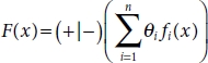
where fi(x) is the weak classifier and θi denotes the calculated weight.
8.5.2.3 Bagging
Bagging is again a tree-ensemble algorithm. It grows decision tree CART models on a subset of the data sample. The decision trees are grown parallely to maximum height and are not pruned. Hence, every tree grown as a part of the ensemble model has high variance and low bias. The CART models vote for a class and the most popular class is chosen. The reason the trees are grown deeper is that the concern of overfitting is less in the bagging algorithm. Therefore, presence of noise does not affect the models performance. The data samples used for growing the trees are randomly selected from the dataset so that the data samples are independent of each other. These are called the bootstrap replica. Fitting these bootstrap samples instead of the entire dataset to the trees increases independence of the sample subsets and thereby decreases output variance.
8.5.3 Neural Network Models
Neural network architecture is collection of interconnected nodes/neurons distributed among different layers like Input layer, hidden layer, and output layer. Based on the number of hidden layers in the architecture the neural network is classified as shallow and deep neural networks. The shallow networks consist of a single hidden layer, whereas deep neural networks consist of two or more hidden layers.
8.5.3.1 Artificial Neural Network (ANN)
ANN [11] is a fundamental model in neural networks which works on the basic concepts of Multi-Level Perceptron (MLP). ANN has a series of inputs (continuous or categorical) each with a designated weight. Each of these weighted inputs are summed over multiple latent layers and finally passed through an activation function that generates an output between 0 and 1 or –1 and 1 depending on the function chosen. An ANN is called a Universal Function Approximator due to its potential to fit any non-linear data. Every layer of the network is densely connected, i.e., every neuron is connected to every other neuron and the inputs are processed only in the forward direction; hence, it is also a Feed-Forward Network. The capability to fit any non-linear model is introduced by the activation function, which helps the network uncover complex associations between the input and the output. But ANN is not suitable for back-propagation, in which the weights of the inputs can be altered to minimize the error function at any layer by propagating back.
8.5.3.2 Convolutional Neural Network (CNN)
CNN [15] is a neural network model usually used for visual image classification but can also be extended to fit other categorical data as well. A CNN consists of a series of densely connected latent layers of weights and filters between the input and the output. As in a regular neural network, the process involves the element-wise dot product of the input with a set of two-dimensional array of weights, called filter. The result obtained as a result of this weighted sum is a two-dimensional feature map. The elements of the feature map are applied to an activation function (ReLU or softmax), which returns a dichotomous result of 0 or 1 indicating the class to which the particular data belongs [20].
8.6 Hyperparameter Tuning
Hyperparameters are external model configurations that are used to estimate model parameters that cannot be directly estimated. Hyperparameter tuning is a method used to choose the best set of values for the model parameters in order to achieve better accuracy. In grid search tuning [10] method, the method is built over a range of parameter values that is specified explicitly by the practitioner in a grid format. It goes over every combination of model parameter values (each given as a list or an array) and picks out the one that has better performance than the rest.
Since it builds and evaluates the model over every possible parameter combination, grid search tuning is exhaustive and deemed computationally expensive.
In contrast, random search randomly picks out points from the hyper-parameter grid and evaluates the model. Also, the number of iterations or the number of combinations to be tried out can be specified externally. This reduces time and the expense of computational power. The best score returned by the random search is based on the randomly chosen hyperpa-rameter grid values, yet this method outperforms Grid Search with comparable accuracy in less time.
8.6.1 Cross-Validation
Cross-validation is a resampling algorithm used to compare different ML models or to find the best tuning parameter for a model. Basically, the data-set is divided into k blocks where k is provided externally, and every block is tested with other blocks as the training set. This is done iteratively for different models [12]. Cross-validation then returns the model that performed the best and with high accuracy. This method helps figure out the best algorithmic model for a given dataset. It is also used in SVM kernels and other similar models for finding hyperparameters.
8.7 Dataset Description
For this study, we used a heart failure clinical dataset containing medical records of patients who had left ventricular systolic dysfunction and with a history of heart failure. The dataset consists of 300 patient’s records from Faisalabad Institute of Cardiology, from April to December 2015. About 64% of the patients in the dataset are Male and the rest 36% are female patients, with their ages ranging between 40 to 95 years old. There are 13 features for each patient in the dataset, out of which 6 features are the clinical variables of the patient like the level of serum creatinine, serum sodium, creatinine phosphokinase, ejection fraction, blood platelets count, and the medical follow-up period of the patients. The target variable in this dataset is the death event feature with binary label, survived patient (death event = 0) and deceased patient (death event = 1). Table 8.1 shows the attributes in the dataset, and Table 8.2 shows the sample dataset taken for analysis.
Table 8.1 Description of each feature in the dataset.
| Feature | Description | Measurement |
| Age | Age of the patient | Years |
| Anemia | Decrease of hemoglobin | Boolean |
| High blood pressure | If a patient is hypotensive | Boolean |
| Creatinine phosphokinase (CPK) | Level of CPK enzyme in the blood | mcg/L |
| Diabetes | If a patient is diabetic | Boolean |
| Ejection fraction (EF) | Percentage of blood leaving heart at each contraction | Percentage |
| Sex | Woman or man | Boolean |
| Platelets | Blood Platelets | Kiloplatelets/ mL |
| Serum creatinine | Level of creatinine in blood | mg/dL |
| Serum sodium | Level of sodium in blood | mEq/L |
| Smoking | If the patient smokes | Boolean |
| Time | Follow-up time of the patient | Days |
| Death event | If the patient died during the follow-up time | Boolean |
Table 8.2 Sample dataset.
| Age | Anemia | Creatinine_phosphokinase | Diabetes | Ejection_fraction | High_bloodpressure | Platelets | Serum_creatinine | Serum_sodium | Sex | Smoking | Time | Death event |
| 75 | 0 | 582 | 0 | 20 | 1 | 265,000 | 1.9 | 130 | 1 | 0 | 4 | 1 |
| 55 | 0 | 7,861 | 0 | 38 | 0 | 263,358.03 | 1.1 | 136 | 1 | 0 | 6 | 1 |
| 65 | 0 | 146 | 0 | 20 | 0 | 162,000 | 1.3 | 129 | 1 | 1 | 7 | 1 |
| 50 | 1 | 111 | 0 | 20 | 0 | 210,000 | 1.9 | 137 | 1 | 0 | 7 | 1 |
| 65 | 1 | 160 | 1 | 20 | 0 | 327,000 | 2.7 | 116 | 0 | 0 | 8 | 1 |
8.7.1 Data Pre-Processing
In this study, the goal is to predict the survival rate of a patient with a history of heart failure and Figure 8.2 shows the complete architecture of the proposed system. There is a moderate class imbalance in these data; only 33% of the records contain information about the deceased patients as shown in Figure 8.3. This imbalance in classes will generate a biased model impacting the analysis. To address the class imbalance problem, we applied SMOTE to increase the number of records in the death event attribute.
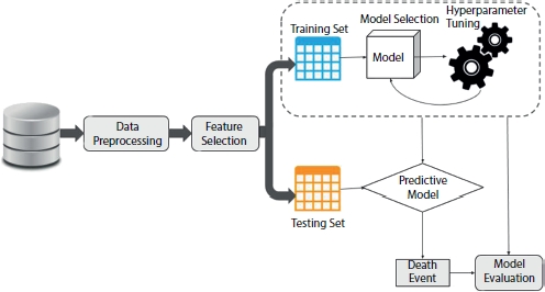
Figure 8.2 Architecture of proposed system.
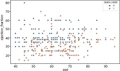
Figure 8.3 Original dataset distribution.
After applying sampling techniques, the number of records is increased to 406 with 203 numbers of entries for each class. Figure 8.4 shows how different SMOTE-based resampling techniques work out to deal with imbalanced data.
Figure 8.5 shows the distribution of target class (DEATH_EVENT) and it is evident from the plot that class 0 is the majority class and class 1 is minority class. After applying SMOTE resampling technique the classes are balanced with 203 records under each class as shown in Figures 8.4 and 8.6.
Figure 8.4 Resampling using SMOTE.
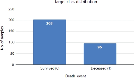
Figure 8.5 Target class distribution.
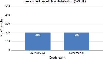
Figure 8.6 Resampled distribution applying SMOTE.
8.7.2 Feature Selection
The dataset consists of 13 attributes of which 3 most relevant features are selected using various feature selection algorithms, Extra Tree Classifier, Forward selection, Chi-square, Pearson Correlation, and Logit model. The Extra Tree Classifier generates the follow-up time, ejection fraction, and serum creatinine as the most important features that influence the survival rate of the heart failure patient as shown in Figure 8.7. Forward feature selection results show that age, ejection fraction, and serum creatinine as the top features.
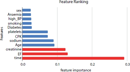
Figure 8.7 Feature ranking using Extra tree classifier.
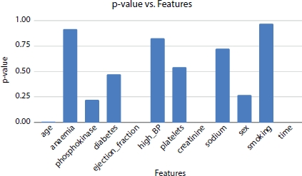
Figure 8.8 p-values of the features.
From Extra Tree Classifier, Pearson Correlation, and Logit model, the hypothesis suggests that time, ejection fraction, and serum creatinine as the top three most significant features. Whereas the other models, Forward Selection and Chi-Square generate that age, ejection fraction, and serum creatinine as the three most significant features. The p-values of ejection fraction, serum creatinine, and time are 0.0 (as shown in Figure 8.8) and are the most significant factors affecting the survival rate of the heart failure patient.
8.7.3 Model Selection
For the analysis, the dataset was split into 80% and 20% of the data as training and testing samples respectively. The model is trained for a two-class problem where the patient’s survival rate is predicted given the medical parameters of the patient. The patient is classified as deceased or survived based on the most important medical features which affect the survival rate of the heart failure patient. The study is divided into three analyses based on the features selected by the various feature selection algorithms. The first study considers the important features predicted by the forward selection algorithm (age, serum creatinine, and ejection fraction). The second study predicts the survival rate of the patient using the attributes which are predicted most important by the Extra Tree Classifier and p-value (time, serum creatinine, and ejection fraction). The third study trains the ML model using all 13 features in the dataset to predict the death event of the patient. The dataset is trained on different ML models and neural networks, Logistic regression, Naive Bayes, SVM, Decision tree, Random forest, K-nearest neighbors, Bagging, AdaBoost, XGBoost, ANN, and Convolutional Neural Network. The hyperparameters of the models are tuned during the learning process using Grid Search and cross- validation techniques to optimize the model and minimize the loss by providing better results. For models such as SVM, neural networks, random forest, and decision trees where hyperparameter tuning is applied, the dataset is split into 70% of training samples, 15% of validation samples, and 15% as testing samples.
8.7.4 Model Evaluation
The classification model can be evaluated with the N × N confusion matrix, where N is the number of classes. The matrix compares the predicted variables and the actual variable to evaluate how well the model performs.
The 2 × 2 matrix contains four values: True Positive (TP), True Negative (TN), False Positive (FP), False Negative (FN). The rows and columns of the matrix represent the actual and predicted values. The confusion matrix for the target variable (Death_Event) is found, and the performance of the supervised models trained is quantified using classification evaluation metrics accuracy and F1-score.
8.8 Experiments and Results
In this section, we elucidate the results obtained for the prediction of survival rate using the three parameters: follow-up time, ejection fraction, and serum creatinine, the results of prediction using age, ejection fraction, and serum creatinine as the dependent features, and the results of prediction using all the features in the clinical records (Table 8.3).
Table 8.3 Experiments description.
| Study | Selected features |
| 1 | All features |
| 2 | Age, ejection fraction, and serum creatinine |
| 3 | Time, ejection fraction, and serum creatinine |
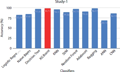
Figure 8.9 Performance evaluation of models under study 1 with dataset size = 1,000.
8.8.1 Study 1: Survival Prediction Using All Clinical Features
The dataset is preprocessed with various pre-processing techniques like applying SMOTE to handle the imbalance in the classes, logarithmic transformations to remove outliers in the features, and applying one hot encoding on the categorical variables to convert them into numerical values. All 12 attributes in the dataset are considered for training them in various ML and DNN classifiers. The prediction shows (Figure 8.9) that XGBoost is the best classifier with 98% accuracy and also correctly predicts the majority of the positive class with accuracy of 94% on the positive class. ANN is the least classifier among all the classifiers with F1-score of 0.60. CNN is found to perform better than ANN which is not the case in the previous study. Table 8.4 shows the accuracy scores of the classifiers that are trained on different sample sizes of dataset. The models show better performance when the data size is upsampled as 1,000 for analysis.
8.8.2 Study 2: Survival Prediction Using Age, Ejection Fraction and Serum Creatinine
The feature age is identified as one of the important features by forward selection feature selection algorithm and chi-square test. The chi-square test exhibits age, ejection fraction, and serum creatinine as the significant features with p-value close to 0. The ML and neural network classifiers are trained with the clinical parameters that are found significant by the chi square test as the predictor variable to predict the survival rate. The performance metrics (Figure 8.10) shows that Bagging is the best classifier for predicting deceased patients with the leading accuracy of 98% and F1-score of 0.97 for data size = 1,000. Among neural network classifiers, outperforms CNN with the accuracy score of 82%, while ANN is the least classifier among all the algorithms with the accuracy score of 77.8%. Table 8.5 shows the accuracy scores of classifiers on different sizes of data and can be interpreted that the performance is increased with increase in size of the dataset.
Table 8.4 Accuracy scores (in %) of all classifiers on different data size.
| Classifiers | Data size = 200 | Data size = 500 | Data size = 1,000 |
| Logistic Regression | 77.3 | 81.51 | 82.48 |
| Naive Bayes | 79.52 | 82.87 | 84.84 |
| Decision Tree | 86.2 | 89.97 | 97.34 |
| XG Boost | 88.7 | 91.7 | 98.92 |
| KNN | 65.76 | 81.33 | 96.5 |
| SVM | 74.83 | 85.2 | 89.56 |
| Random Forest | 88.16 | 89.87 | 97.24 |
| AdaBoost | 86.9 | 85.2 | 91.3 |
| Bagging | 86.43 | 88.64 | 98.72 |
| ANN | 60.91 | 84.84 | 69.17 |
| CNN | 78.66 | 80.3 | 86.43 |
8.8.3 Study 3: Survival Prediction Using Time, Ejection Fraction, and Serum Creatinine
The follow-up time, ejection fraction, and serum creatinine were obtained as the top three important features that affect the survival rate of the heart failure patient using extra tree classifier. The statistics of logit model is also used to find the feature importance with respect to the response variable. The logit statistics test showed that the p-value is close to 0 for time, ejection fraction, and serum creatinine. These three features are used as the predictor variables in predicting the death event of the patient. The dataset is balanced using the SMOTE algorithm and then trained using various ML models. For models such as SVM, decision tree, CNN, ANN, KNN, and random forest, the dataset is split into 70% for training, 15% for validation, and 15% for testing. The hyperparameters for these models are selected using the Grid Search algorithm in order to get the optimized result. For other models like Naive Bayes, XGBoost, AdaBoost, Bagging, and logistic regression classifiers, the data is split into 80% for training and 20% for testing.
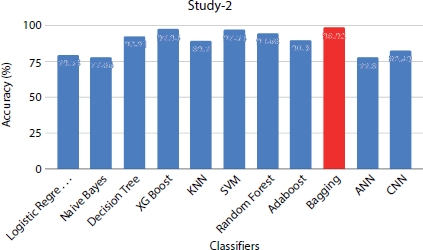
Figure 8.10 Performance evaluation of models under study 2 with data size = 1,000.
Table 8.5 Accuracy scores (in %) of all classifiers on different data size.
| Classifiers | Data size = 200 | Data size = 500 | Data size = 1,000 |
| Logistic Regression | 73.87 | 69.1 | 79.53 |
| Naive Bayes | 73.67 | 72.47 | 77.86 |
| Decision Tree | 80.3 | 82.49 | 92.91 |
| XG Boost | 79.6 | 84.85 | 97.94 |
| KNN | 79.79 | 80.1 | 89.7 |
| SVM | 79.08 | 84.44 | 97.54 |
| Random Forest | 81.25 | 86.03 | 94.68 |
| AdaBoost | 77.1 | 77.8 | 90.3 |
| Bagging | 80.52 | 88.57 | 98.92 |
| ANN | 77.08 | 63.4 | 77.8 |
| CNN | 62.6 | 74.93 | 82.49 |
Table 8.6 Accuracy scores (in %) of all classifiers on different data size.
| Classifiers | Data size = 200 | Data size = 500 | Data size = 1,000 |
| Logistic Regression | 73.87 | 81.51 | 82.48 |
| Naive Bayes | 73.67 | 82.87 | 84.55 |
| Decision Tree | 80.3 | 89.97 | 96.65 |
| XG Boost | 79.6 | 91.7 | 99.11 |
| KNN | 79.79 | 81.33 | 92.7 |
| SVM | 79.08 | 85.2 | 97.44 |
| Random Forest | 81.25 | 89.87 | 95.96 |
| AdaBoost | 77.1 | 85.2 | 90.3 |
| Bagging | 80.52 | 88.64 | 98.92 |
| ANN | 77.08 | 84.84 | 85.5 |
| CNN | 62.6 | 80.3 | 88.16 |
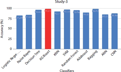
Figure 8.11 Performance evaluation of models under study 3 With dataset size = 1,000.
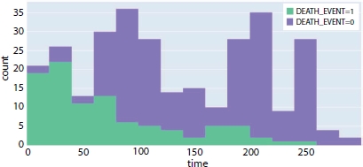
Figure 8.12 Correlation between follow-up time and death event.
Among the ML models (Table 8.6), XGBoost classifier and Bagging classifier outperform other models with highest accuracy of 99% and top F1-score of 0.96 when the dataset size is 1,000. Naive Bayes achieved a top accuracy of 92% and correctly classified the majority of the survived patients (49/53) than any other classifier. Random forest predicts correctly the majority of the patients who have less chance of survival achieving an accuracy of 82% on the positive class. The Convolution Neural Network and ANN obtain the accuracy of 80% and 84%, respectively. The ANN is the least performing classifier with an accuracy of 85%. Figure 8.11 shows the performance metrics comparison among all the models which are trained with sample size of 1,000 records.
Table 8.7 Logit model statistical test.
| Features | p-value |
| Age | 0.07 |
| Anemia | 0.39 |
| Phosphokinase | 0.04 |
| Diabetes | 0.98 |
| Ejection_fraction | 0.00 |
| High_BP | 0.27 |
| Platelets | 0.15 |
| Creatinine | 0.00 |
| Sodium | 0.20 |
| Sex | 0.96 |
| Smoking | 0.86 |
| Time | 0.00 |
Table 8.8 Chi-square test.
| Features | p-value |
| Age | 0.000 |
| Anemia | 0.9178 |
| Phosphokinase | 0.2203 |
| Diabetes | 0.4751 |
| Ejection_fraction | 0 |
| High_BP | 0.8282 |
| Platelets | 0.545 |
| Creatinine | 0.0001 |
| Sodium | 0.7225 |
| Sex | 0.2727 |
| Smoking | 0.9677 |
| Time | 0.007 |
Though the classifiers perform well given time, ejection fraction, and serum creatinine as the medical features for predicting the survival rate, the correlation between the follow-up time and the patient’s survival rate is investigated. Figure 8.12 shows that, as the follow time increases, the patients who have deceased (Death_event = 1) is very minimum compared to the patients at the initial trial of medication. Even though there is no complete linear correlation between the follow-up time and the survival rate, it is one of the important parameters and cannot be eliminated completely. The p-values obtained using statistical Logit model is shown in Table 8.7 and chi-square test values for study-2 is depicted in Table 8.8.
8.8.4 Comparison Between Study 1, Study 2, and Study 3
Supervised models like Logistic regression, Naive Bayes, Decision Tree, KNN, and SVM perform better when extra tree classifier is used for feature selection (study 3) compared to the other two studies (Figure 8.13). Among neural network classifiers, ANN performs least when all features are considered for training, and the highest performance is seen in the study 3, while CNN is the least performer in the study 2 but brings about comparatively better results in study 1 and study 3. Ensemble models like XGBoost, Random Forest, and Bagging show a best performance for all the three studies irrespective of the features considered for training. Overall, all models used for prediction perform extremely well when they are trained with time, ejection fraction, and serum creatinine as the predictor variables. In most of the cases, the models do not perform well when age is considered as one of the features. The findings from the statistical and performance analysis show that age may not be a significant factor which affects the survival rate of the patient. Also, other factors like cholesterol, high blood pressure, and smoking are not found to be significant factors that affect the survival rate of the heart failure patient. One of the ground causes of this may be these factors are basically the features which influence heart failure at the early stage, but this study is concerned with the patients at the advanced level of heart failure. The first study, i.e., the one with follow-up time, serum creatinine, and ejection fraction, showed maximum accuracy thereby implying the influence of these factors on a CVD patient’s survival.
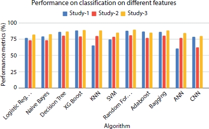
Figure 8.13 Performance evaluation of models on different classifiers.
8.8.5 Comparative Study on Different Sizes of Data
To analyze how the size of the dataset affects the model performance, the initial dataset containing 299 records is upsampled to 508 and 1,000 using upsampling technique to account for the problem of data imbalance.
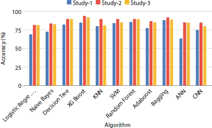
Figure 8.14 Performance evaluation of models on dataset size = 508.
Figure 8.14 shows that there is a significant increase in the accuracy of the trained models when the dataset is increased to 508. XGBoost ensemble model which outperforms in the previous analysis (Figure 8.13) shows the same nature when the dataset size is increased with the accuracy score elevating to 93%. In neural network classifier models, there is an increase in trend when the dataset size is increased. To further improve the quality and precision of the model, the sample size is increased to 1,000. Figure 8.15 shows the accuracy results obtained by all the classification algorithms on the three different studies when trained with the number of records in the dataset upsampled to 1,000 records. It is observed that the models perform best in precision and accuracy when the sample size of the data is increased. Classifiers like decision tree, bagging, and SVM give exceedingly good results compared to previous analysis using smaller dataset.
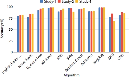
Figure 8.15 Performance evaluation of models on dataset size = 1,000.
8.9 Analysis
There is no universal model that performs best for the whole pool of datasets available for analysis. The prediction and the performance of the model depend on the nature and quality of the dataset on which the model is trained. From our analysis, it shows that the ensemble models XGBoost and random forest out performs the baseline ML algorithms and neural networks for the considered dataset. The tree-based model gives a decent result in a fast manner, whereas neural networks lack the one reason for this contusion that is the size of the data. Neural networks like CNN require a large and feature engineered dataset to train on and hypertuned parameters to outperform in the evaluation. With increasing dataset, the performance of CNN is also observed to be increasing, but XGBoost gives the desired results with 1,000 records itself and further increasing the dataset samples may cause the ML models to overfit even though neural networks may see an increasing trend. Hence, ensemble and ML classifier models are adequate for the prediction of survival rate of the heart failure patient with minimum resources and reduced time complexity.
8.10 Conclusion
Our work employs various feature selection techniques and classification algorithms to predict the survival rate of the heart failure patient. This approach not only helps us predict the survival rate of a patient but also in early prognosis of those that are more likely to develop CVDs and in that process give the physicians a headstart in treating the patients. Based on the features selected by the feature selection techniques, three studies are carried out and the performance of the models trained are evaluated for all the studies. Study 1 trains all the features in the dataset. Study 2 uses features selected using forward selection techniques: age, serum cre-atinine, and ejection fraction. Study 3 consists of features follow-up time, serum creatinine, and ejection fraction selected using extra tree classifier. The classification models are applied on the features selected in each study. From the results obtained in the study, it is interpreted that XGBoost and random forest from the ensemble model are the overall best performers in all three studies for the given heart failure dataset. Study 3 which applies time, serum creatinine, and ejection fraction as the most important features performs best on all classification models compared to other two studies. Furthermore, to enhance the performance of the classifiers, all three studies are repeated on different dataset sizes, and it is observed that XGBoost performs well in this case also.
This work concentrates on the static data of heart failure patients collected from the clinical trial; furthermore, this work can be extended to real-time monitoring of patients using mobile application. Real-time monitoring of patient’s clinical features using wearable devices can be a supportive technology for doctors with less experience in that subject matter and also for the patients and their family for the early detection of heart failure.
References
1. Adler, E.D., Voors, A.A., Klein, L., Macheret, F., Braun, O.O., Improving risk prediction in heart failure using machine learning. Eur. J. Heart Fail., 22, 1, 139–147, 2020, 10.1002/ejhf.1628.
2. Ahmad, T., Munir, A., Bhatti, S.H., Survival analysis of heart failure patients: A case study. PLoS One, 12, 7, 2017.
3. Alasadi, S.A. and Bhaya, W.S., Review of data pre-processing techniques in data mining. J. Eng. Appl. Sci., 12, 16, 4102–4107, 2017, 10.3923/jeasci.2017.4102.4107.
4. Angraal, S., Mortazavi, B.J., Gupta, A., Khera, R., Ahmad, T., Desai, N.R., Jacoby, D.L., Machine Learning Prediction of Mortality and Hospitalization in Heart Failure With Preserved Ejection Fraction. JACC: Heart Fail., 8, 1, 12–21, 2020, 10.1016/j.jchf.2019.06.013.
5. Bennett, J.A., Riegel, B., Bittner, V., Nichols, J., Validity and reliability of the NYHA classes for measuring research outcomes in patients with cardiac disease. Heart Lung: J. Acute Crit. Care, 31, 4, 62–70, 10.1067/mhl.2002.124554.
6. Borlaug, B.A., Evaluation and management of heart failure with preserved ejection fraction. Nat. Rev. Cardiol., 17, 9, 559–573, 2020, 10.1038/s41569-020-0363-2.
7. Charlene, B., Margherita, M., Alexander, K., Rafael, A.-G., Lorna, S., New York Heart Association (NYHA) classification in adults with congenital heart disease: Relation to objective measures of exercise and outcome. Eur. Heart J. – Qual. Care Clin. Outcomes, 4, 1, 51–58, 2018, 10.1093/ehjqcco/qcx031.
8. Chicco, D. and Jurman, G., Machine learning can predict survival of patients with heart failure from serum creatinine and ejection fraction alone. BMC Med. Inf. Decis. Making, 20, 1, 2020, 10.1186/s12911-020-1023-5.
9. Chiew, C.J., Liu, N., Tagami, T., Wong, T.H., Heart rate variability based machine learning models for risk prediction of suspected sepsis patients in the emergency department. Med. (United States), 98, 6, 2019.
10. Hatem, F.A. and Amir, A.F., Speed up grid-search for parameter selection of support vector machines. Appl. Soft Comput. J., 80, 202–210, 2019, 10.1016/j. asoc.2019.03.037.
11. Javeed, A., Rizvi, S.S., Zhou, S., Riaz, R., Khan, S.U., Kwon, S.J., Heart risk failure prediction using a novel feature selection method for feature refinement and neural network for classification. Mob. Inf. Syst., 2020, 2020, 10.1155/2020/8843115.
12. Mary, B., Brindha, G.R., Santhi, B., Kanimozhi, G., Computational models for predicting anticancer drug efficacy: A multi linear regression analysis based on molecular, cellular and clinical data of Oral Squamous Cell Carcinoma cohort. Comput. Methods Programs Biomed., 178, 105–112, 2019, 10.1016/j.cmpb.2019.06.011.
13. Nithya, R. and Santhi, B., Comparative study on feature extraction method for breast cancer classification. J. Theor. Appl. Inf. Technol., 31, 2, 220–226, 2011.
14. Nithya, R. and Santhi, B., Mammogram classification using maximum difference feature selection method. J. Theor. Appl. Inf. Technol., 33, 2, 197–204, 2011.
15. Nithya, R. and Santhi, B., Breast cancer diagnosis in digital mammograms using statistical features and neural networks. Res. J. Appl. Sci. Eng. Tech., 4, 24, 5480–5483, 2012.
16. Nithya, R. and Santhi, B., Decision tree classifiers for mass classification. Int. J. Signal Imaging Syst. Eng., 8, 1–2, 39–45, 2015, 10.1504/IJSISE.2015.067068.
17. Nithya, R. and Santhi, B., Application of texture analysis method for mammogram density classification. J. Instrum., 12, P07009–P07009, 2017, 10.1088/1748-0221/12/07/P07009.
18. Packer, M., What causes sudden death in patients with chronic heart failure and a reduced ejection fraction. Eur. Heart J., 41, 18, 15229645, 2020.
19. Pfeffer, M.A., Shah, A.M., Borlaug, B.A., Heart Failure with Preserved Ejection Fraction in Perspective. Circ. Res., 124, 11, 1598–1617, 2019, 10.1161/CIRCRESAHA.119.313572.
20. Rishiikeshwer, S., Shriram, T., Raju, J., Hari, M., Santhi, B., Brindha, G.R., Farmer-Friendly Mobile Application for Automated Leaf Disease Detection of Real-Time Augmented Data Set using Convolution Neural Networks. J. Comput. Sci., 16, 158–166, 2020, 10.3844/jcssp.2020.158.166.
21. Saeys, Y., Abeel, T., Van De Peer, Y., Robust feature selection using ensemble feature selection techniques. Lect. Notes Comput. Sci. (including subseries Lecture Notes Artificial Intelligence and Lecture Notes in Bioinformatics), 5212 LNAI, PART 2, 313–325, 2008, 10.1007/978-3-540-87481-2_21.
22. Shakthi, K.P.A., Brindha, G.R., Bharathi, N., Enhanced classification through improved feature selection technique. Int. J. Mech. Eng. Technol., 8, 10, 342–351, 2017.
23. Suresh, A., Aashish, S., Santhi, B., Multi classifier analysis using data mining classification algorithms. Int. J. Appl. Eng. Res., 9, 22, 13047–13060, 2014.
24. Taha, K., An Ensemble-based approach to the development of clinical prediction models for future-onset heart failure and coronary artery disease using machine learning. J. Am. Coll. Cardiol., 75, 11, 2046, 2020.
25. Timmis, A., Townsend, N., Gale, C., Torbica, A., Lettino, M., European society of cardiology: Cardiovascular disease statistics 2019. Eur. Heart J., 41, 1, 12–85, 2020, 10.1093/eurheartj/ehz859.
26. Wang, Z., Zhu, Y., Li, D., Yin, Y., Zhang, J., Feature rearrangement based deep learning system for predicting heart failure mortality. Comput. Methods Programs Biomed., 191, 2020, 10.1016/j.cmpb.2020.105383.
27. Yan, Y., Liu, R., Ding, Z., Du, X., Chen, J., Zhang, Y., A parameter-free cleaning method for SMOTE in imbalanced classification. IEEE Access, 7, 23537–23548, 2019, 10.1109/ACCESS.2019.2899467.
- *Corresponding author: [email protected]