
14
Measuring Urban Sprawl Using Machine Learning
Keerti Kulkarni* and P. A. Vijaya
Dept of ECE, BNM Institute of Technology, Bangalore, India
Abstract
Urban sprawl generally refers to the amount of concrete jungle in a given area. In the present context, we consider a metropolitan area of Bangalore. The area has grown tremendously in the past few years. To find out how much of the area is occupied by built-up areas, we consider the remotely sensed images of the Bangalore Urban District. Each material on the earth’s surface reflects a different wavelength, which is captured by the sensors mounted on a satellite. In short, the spectral signatures are the distinguishing features used by the machine learning algorithm, for classifying the land cover classes. In this study, we compare and contrast two types on machine learning algorithms, namely, parametric and non-parametric with respect to the land cover classification of remotely sensed images. Maximum likelihood classifiers, which are parametric in nature, are 82.5% accurate for the given study area, whereas the k-nearest neighbor classifiers give a better accuracy of 85.9%.
Keywords: Urbanization, maximum likelihood classifier, support vector machines, remotely sensed images
14.1 Introduction
Urbanization is a key deciding factor for the government to provide various infrastructure facilities. It is an indirect indication of the amount of population staying in the cities. Although the census report does provide this information, it is generally a very tedious process. Remotely sensed images aid this kind of an analysis, wherein we try to classify the raw images and extract the built-up areas from it. Machine learning algorithms have been traditionally used for the classification of the land cover. We basically need the features depending on which the classification can be done. We also need distance measures, to calculate how far apart the features in the feature space are. In Section 14.2, a brief literature survey of the various methodologies used here is given. Section 14.3 describes the basics of remotely sensed images and the pre-processing done. The main emphasis is on the machine learning algorithms and not on the images themselves; hence, only basics related to these images are provided. Section 14.4 deals with features and their selection criteria. The different methods of calculating distances and similarities along with the equations are given, as these form a basis for feature selection. In Section 14.5, the emphasis is on the machine learning classifiers as applicable to the work. Section 14.6 details and compares the results obtained. We finally discuss the results and conclude in Section 14.7.
14.2 Literature Survey
The literature survey was undertaken on two levels. One domain is related to understand the remote sensing images, the band information, and the pre-processing that is required. The other relates to the various machine learning algorithms that can be used for the land cover classification.
Satellite images can be multispectral or hyperspectral. Hyperspectral images have a greater number of overlapping bands, whereas multispectral images have a smaller number of non-overlapping bands. Both the types can be used for wetland mapping [1]. This can be extended to the land use classification also. Pre-processing of the multispectral images, including atmospheric correction and enhancement techniques have been discussed by various authors [2, 3]. Geometric processing may also be required in certain datasets and applications [4]. The datasets which we use have been geometrically corrected.
The next literature survey was to analyze the pros and cons and comparisons of various machine learning algorithms [5, 6]. Maximum likelihood classifier (MLC) algorithm has been used and compared with regression trees for estimating the burned areas of the grassland [7]. MLC has been used for sea ice mapping of the polarimetric SAR images [8]. MLC has also been used to compare the outputs from two different datasets Landsat and SAR images [9] and land cover changes integrated with GIS [10]. Additional metadata or the Normalized Difference Vegetation Indices (NDVI) is used with the classification algorithms to improve the accuracy of classification [11, 12]. Use of Normalized Difference Built-up Index (NDBI) for the calculation of urban sprawl is discussed by the authors in [13]. Urbanization is directly related to the land surface temperature [14, 15]. The land cover change can also be analyzed using Adaptive Neuro Fuzzy Inference Systems [16]. Object-based classification methods as compared to pixel-based classification have been discussed by various authors [17, 18]. The evaluation methods for the machine learning models have been discussed [19, 20].
14.3 Remotely Sensed Images
The images captured from the cameras mounted on a satellite are generally termed as remote sensing images. In this work, we have used the LANDSAT-8 images captured in 2019. The dataset is freely downloadable from the GloVis website. The Landsat images have nine spectral bands and two thermal bands. Out of these eight spectral bands have a resolution of 30 meters and one band (band 8) has a resolution of 15 meters. Two of the bands in the raw form, as downloaded, are shown in Figure 14.1. The thermal bands (Band 10 and Band 11) have a resolution of 100 meters. Out of these bands, we choose bands 2-7 as the features, because of their distinct spatial signatures. In other words, these bands used in different combination can easily distinguish between the different land cover classes. As an example, the band combination 3-4-6 is good for visualizing urban environments. Here, the vegetation is shown in green, and water is dark blue or black. The built-up areas generally show up as brown. The band combinations are shown in Figure 14.2. Comparing Figures 14.1 and 14.2, we can make out how using a combination of the bands aids the visualization.
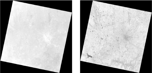
Figure 14.1 Raw images (Band 2 and Band 5, respectively).
The images have to be preprocessed for atmospheric corrections before they can be further used. We have chosen only those image sets where the cloud cover is less than 10%. Hence, correction for cloud removal is not required. Further, atmospheric correction provides a kind of normalization of the spectral signatures, which makes them easily distinguishable in the feature space. Figure 14.3 shows the spectral signatures after the atmospheric correction.
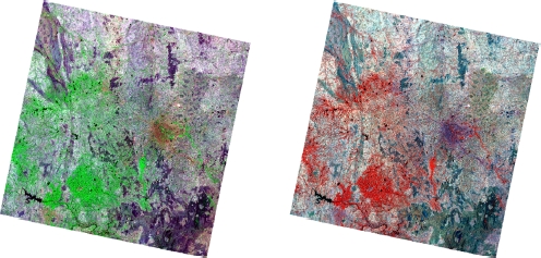
Figure 14.2 Band combination 3-4-6 and 3-2-1, respectively.
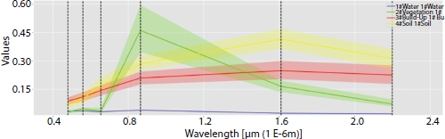
Figure 14.3 Spectral signatures after atmospheric correction.
14.4 Feature Selection
Feature selection is based on the spectral distances. Distance-based metrics as compared to similarity-based metrics are of better use for the selection of features. Similarity-based metrics give the degree of similarity between the vectors, whereas the distance-based metrics tell us how different the features are from each other.
14.4.1 Distance-Based Metric
The spectral distances evaluate the degree of separability between the spectral signatures. The Euclidean distance is one of the simplest methods for calculating the separability. In its simplest form, the Euclidean distance gives the degree of separability in an N-dimensional vector space. The more the distance, the better is the separability. If the Euclidean distance is zero, then the spectral signatures are same and hence cannot be used as feature. The better the separability, the more will be the Euclidean distance. Mathematically,
where
x = first spectral signature vector;
y = second spectral signature vector;
n = number of image bands under consideration.
The other distance-based metric that can be used is the Manhattan distance, which is given as
Figure 14.4 shows the difference between the Euclidean distance and the Manhattan distance. The green line represents the Euclidean distance, and the red line represents the Manhattan distance. Manhattan distance is preferred when we have a high-dimensional dataset, where it gives better results compared to the Euclidean distance. As shows from the figure, the Euclidean distance seems to be better suited for the application in hand; hence, we use it for feature selection.
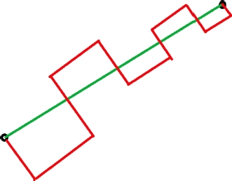
Figure 14.4 Pictorial representation of Euclidean and Manhattan distances.
14.5 Classification Using Machine Learning Algorithms
14.5.1 Parametric vs. Non-Parametric Algorithms
Parametric algorithms are the ones, which use a fixed set of parameters, and we assume that the data follows a specified probability distribution (e.g., MLC). Even if the training data is increased, there is no guarantee that the accuracy of the algorithm will improve. On the other hand, the complexity of a non-parametric [e.g., support vector machine, k-nearest neighbor (k-NN)] model will increase with number of parameters.
14.5.2 Maximum Likelihood Classifier
We have a large number of sample points available with us, since the dataset is really huge. Hence, the MLC works best according to literature. The likelihood function tells us how likely the observed pixel is as a function of the possible classes. Maximizing this likelihood outputs the class that agrees with that pixel most of the time. Mathematically, maximum likelihood algorithm calculates the probability distributions for the classes, related to Bayes’ theorem, estimating if a pixel belongs to a land cover class. In order to use this algorithm, a sufficient number of pixels are required for each training area, allowing for the calculation of the covariance matrix. The discriminant function is calculated for every pixel as given in Equation (14.3):
where
Ck = land cover class k;
x = spectral signature vector of an image pixel;
p(Ck) = probability that the correct class is Ck;
|Σ k| = determinant of the covariance matrix of the data in class Ck;
![]() inverse of the covariance matrix k
inverse of the covariance matrix k
yk = spectral signature vector of class k.
Therefore,
Figure 14.5 shows the intuitive approach toward this kind of a classification. The two curves can be considered as two different classes with distinct discriminant functions. Here, since we have four classes, we will have four such distinct curves.
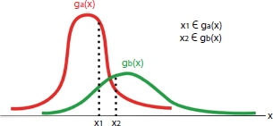
Figure 14.5 Discriminant functions.
14.5.3 k-Nearest Neighbor Classifiers
The k-NN algorithm simply considers all the sample points together and classifies them depending on the similarity measures. The similarity (or dissimilarity) measures can be calculated by using the Euclidean distance mentioned before in Section 14.3. The important parameter to be considered in the k-NN implementation is the value of k. The value of k decides how many neighbors we consider for the classification. For example, if we keep k = 5, then we consider the output from majority voting of 5 neighbors. A smaller value of k is susceptible to noise, whereas a larger value is computationally expensive. The value of k also depends on the training data size. Here, we have roughly 2,500 pixels belonging to different classes as a training data. Hence, we choose k = sqrt(2,500) = 50.
14.5.4 Evaluation of the Classifiers
The evaluation of both the algorithms is done by the chalking out the confusion matrix that represents the output of the classification algorithm. Generally, for a two-class problem, the confusion matrix looks as shown in Table 14.1.
The confusion matrix is used to indicate the performance of the model on the test data, for which the true values are known. Depending on these values, we obtain the precision, recall, and the F-score values for that model.
14.5.4.1 Precision
Precision expresses the proportion of pixels that the model says belongs to Class A, actually belongs to Class A. Referring to the confusion matrix in Table 14.1, mathematically,
Table 14.1 General confusion matrix for two class problems.
| Class 1 predicted | Class 2 predicted | |
| Class 1 Actual | TP | FN |
| Class 2 Actual | FP | TN |
14.5.4.2 Recall
Recall indicates the relevance of the pixels classified. In other words, it is a measure of the model’s ability to identify true positives. It is also called as sensitivity or true positive rate.
14.5.4.3 Accuracy
Using accuracy is intuitive. It is an indication of how correct the model is. In other words, all trues divided by all the values in the confusion matrix.
14.5.4.4 F1-Score
There are certain instances, where the trade-off between precision and recall is required. In some other instances, both of them are actually important. In these cases, F1-score is a better measure. It is a harmonic mean of precision and recall.
14.6 Results
As mentioned previously, the remotely sensed images were preprocessed and then classified. Figure 14.6 shows the results of the MLC and Figure 14.7 shows the output of the kNN Classifier. Note then, the actual satellite image was very large. It has been clipped to show only the region of interest, in this case, the area in and around Bangalore. The red color shows the concentration of the urban or the built-up areas. Other land cover classes are indicated accordingly in the legend. The confusion matrices obtained from the MLC and the k-NN classifier are shown in Tables 14.2 and 14.3, respectively. Table 14.4 shows the average precision, recall, F1-score, and accuracy of both the methods.
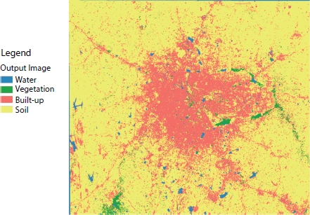
Figure 14.6 Result of ML classifier.
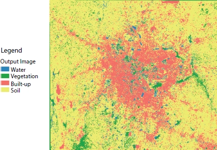
Figure 14.7 Result of k-NN classifier.
Observe that in both the cases, we get a better score for the precision, but the value for recall is less. There is always a trade-off between the two. Here, the precision is of more importance for which we get a value of 82% for the MLC and a value of 86% for the k-NN. Also, the accuracy of the k-NN is better (85.9%) compared to that of the MLC (82.5%).
Table 14.2 Confusion matrix for a ML classifier.
| Water | Vegetation | Built-up | Soil | |
| Water | 194 | 15 | 5 | 6 |
| Vegetation | 20 | 152 | 8 | 22 |
| Built-Up | 2 | 10 | 188 | 3 |
| Soil | 32 | 21 | 7 | 178 |
Table 14.3 Confusion matrix for a k-NN classifier.
| Water | Vegetation | Built-up | Soil | |
| Water | 200 | 14 | 2 | 8 |
| Vegetation | 20 | 162 | 2 | 12 |
| Built-Up | 8 | 6 | 195 | 4 |
| Soil | 20 | 16 | 9 | 185 |
Table 14.4 Average precision, recall, F1-score, and accuracy.
| Precision | Recall | F1-score | Accuracy | |
| ML | 0.826364 | 0.25 | 0.383366 | 0.825029 |
| k-NN | 0.861825 | 0.25 | 0.387078 | 0.859791 |
14.7 Discussion and Conclusion
As seen from Figures 14.6 and 14.7, both the classifiers give comparable results. The built-up part, which is shown in red color, is concentrated in the center of the city, which is justified since much of the urban activities are in and around this area. The MLC output shows continuous areas of red, whereas the k-NN output shows red areas interspersed with the yellow, blue, and green areas, especially in the middle part of the image. This indicates that the k-NN algorithm is capable of finer classification compared to the MLC. Comparison with the ground truth (survey maps) also ascertains this fact.
The complexity and the running time of the algorithm for the MLC are independent of the changes in any of the parameters (number of training pixels). The complexity and the running time of the k-NN increases with the increase in number of training pixels. This directly increases the k value and the algorithm has to look at a greater number of neighbors for the classification of the pixels. This increases the time taken for generating the model. On the plus side, a higher value of k generates a land cover map which is nearer to the ground truth.
We conclude by saying that the accuracy and the efficiency of the algorithms depend majorly on the feature set used. It also depends on the domain knowledge of the user and the dataset used for the classification. Choosing a proper machine learning algorithm to better suit the classification problem is a critical part of the entire process of classification.
As a future work, some more non-parametric classifiers like support vector machines and random forests can be explored. A still further extension can be the use of convolutional neural networks, which are patch-based, as opposed to pixel-based used here. This may further increase the accuracy.
Acknowledgements
The authors extend a heartfelt thanks to the management of BNM Institute of Technology, Bangalore, for providing us the infrastructure to carry out the research work on which this publication is based. The authors also sincerely thank Visveswaraya Technological University for providing the platform to do the research work.
References
1. Adam, E., Mutanga, O., Rugege, D., Multispectral and hyperspectral remote sensing for identification and mapping of wetland vegetation: A review. Wetl. Ecol. Manage., 18, 281–296, 2010, https://doi.org/10.1007/s11273-009-9169-z.
2. K. Themistocleous, D. G. Hadjimitsis, D. G. Hadjimitsis, and K. Themistocleous, The importance of considering atmospheric correction in the pre-processing of satellite remote sensing data intended for the management and detection of cultural sites: a case study, Proceedings of the 14th International Conference on Virtual Systems and Multimedia, pp 9–12, October, 2008.
3. Hanspal, R.K. and Sahoo, K., A Survey of Image Enhancement Techniques. Int. J. Sci. Res., 6, 2467–2471, 2017.
4. Toutin, T., Geometric processing of remote sensing images: Models, algorithms and methods. Int. J. Remote Sens., 25, 1893–1924, 2004, https://doi.org/10.1080/0143116031000101611.
5. Talukdar, S., Singha, P., Mahato, S., Shahfahad, Pal, S., Liou, Y.A., Rahman, A., Land-use land-cover classification by machine learning classifiers for satellite observations-A review. Remote Sens., pp 1–24 12, 2020, https://doi.org/10.3390/rs12071135.
6. Nitze, I., Schulthess, U., Asche, H., Comparison of machine learning algorithms random forest, artificial neuronal network and support vector machine to maximum likelihood for supervised crop type classification. Proc. 4th Conf. Geogr. Object-Based Image Anal. – GEOBIA 2012, pp. 35–40, 2012.
7. Cabral, A.I.R., Silva, S., Silva, P.C., Vanneschi, L., Vasconcelos, M.J., ISPRS Journal of Photogrammetry and Remote Sensing Burned area estimations derived from Landsat ETM + and OLI data: Comparing Genetic Programming with Maximum Likelihood and Classification and Regression Trees. ISPRS J. Photogramm. Remote Sens., 142, 94–105, 2018, https://doi.org/10.1016/j.isprsjprs.2018.05.007.
8. Dabboor, M. and Shokr, M., ISPRS Journal of Photogrammetry and Remote Sensing A new Likelihood Ratio for supervised classification of fully polarimetric SAR data : An application for sea ice type mapping. ISPRS J. Photogramm. Remote Sens., 84, 1–11, 2013, https://doi.org/10.1016/j.isprsjprs.2013.06.010.
9. Ali, M.Z., Qazi, W., Aslam, N., The Egyptian Journal of Remote Sensing and Space Sciences A comparative study of ALOS-2 PALSAR and landsat-8 imagery for land cover classification using maximum likelihood classifier. Egypt. J. Remote Sens. Space Sci., 21, S29–S35, 2018, https://doi.org/10.1016/j.ejrs.2018.03.003.
10. Mishra, P.K., Rai, A., Rai, S.C., Land use and land cover change detection using geospatial techniques in the Sikkim Himalaya, India. Egypt. J. Remote Sens. Space Sci., 23, 2, 133–143, 2019, https://doi.org/10.1016/j.ejrs.2019.02.001.
11. Taufik, A., Ahmad, S.S.S., Ahmad, A., Classification of Landsat 8 satellite data using NDVI thresholds. J. Telecommun. Electron. Comput. Eng., 8, 4, 37–40, 2016.
12. Wen, Z., Wu, S., Chen, J., Lü, M., NDVI indicated long-term interannual changes in vegetation activities and their responses to climatic and anthropogenic factors in the Three Gorges Reservoir Region, China. Sci. Total Environ., 574, 947–959, 2017, https://doi.org/https://doi.org/10.1016/j.scitotenv.2016.09.049.
13. Krishna, H., Study of normalized difference built-up (NDBI) index in automatically mapping urban areas from Landsat TM imagery. Int. J. Eng. Sci., 7, 1–8, 2018.
14. Guha, S., Govil, H., Gill, N., Dey, A., A long-term seasonal analysis on the relationship between LST and NDBI using Landsat data. Quat. Int., 575–576, 249–258, 2020, https://doi.org/https://doi.org/10.1016/j.quaint.2020.06.041.
15. Debnath, M., Syiemlieh, H.J., Sharma, M.C., Kumar, R., Chowdhury, A., Lal, U., Glacial lake dynamics and lake surface temperature assessment along the Kangchengayo-Pauhunri Massif, Sikkim Himalaya, 1988–2014. Remote Sens. Appl. Soc. Environ., 9, 26–41, 2018, https://doi.org/https://doi.org/10.1016/j.rsase.2017.11.002.
16. Sivagami, K.P., Jayanthi, S.K., Aranganayagi, S., Monitoring Land Cover of Google Web Service Images through ECOC and ANFIS Classifiers, 5, 8, 9–16 2017.
17. Rizvi, I.A. and Mohan, B.K., Object-based image analysis of high-resolution satellite images using modified cloud basis function neural network and probabilistic relaxation labeling process. IEEE Trans. Geosci. Remote Sens., 49, 12, 4815–4820, 2011, https://doi.org/10.1109/TGRS.2011.2171695.
18. Qian, Y., Zhou, W., Yan, J., Li, W., Han, L., Comparing Machine Learning Classifiers for Object-Based Land Cover Classification Using Very High Resolution Imagery. 7, 153–168, 2015, https://doi.org/10.3390/rs70100153.
19. Deborah, H., Richard, N., Hardeberg, J.Y., A Comprehensive Evaluation of Spectral Distance Functions and Metrics for Hyperspectral Image Processing. IEEE J. Sel. Top. Appl. Earth Obs. Remote Sens., 8, 3224–3234, 2015, https://doi.org/10.1109/JSTARS.2015.2403257.
20. Pontius, R.G. and Millones, M., Death to Kappa: Birth of quantity disagreement and allocation disagreement for accuracy assessment. Int. J. Remote Sens., 32, 4407–4429, 2011, https://doi.org/10.1080/01431161.2011.552923.
- *Corresponding author: [email protected]