The true beauty and amazing power of TCP/IP lies in one word: routing. Routing enables us to interconnect individual LANs into WANs. Routers, the magic boxes that act as the interconnection points, have all the built-in smarts to inspect incoming packets and forward them toward their eventual LAN destination. Routers are, for the most part, automatic. They require very little in terms of maintenance once their initial configuration is complete because they can talk to each other to determine the best way to send IP packets.

This chapter discusses how routers work, including an in-depth look at different types of network address translation (NAT), and then dives into an examination of various dynamic routing protocols such as Open Shortest Path First (OSPF) and Border Gateway Protocol (BGP). The chapter finishes with the nitty-gritty details of installing and configuring a router successfully. Not only will you understand how routers work, you should be able to set up a router and diagnose common router issues by the end of this chapter.

Historical/Conceptual

How Routers Work

A router is any piece of hardware or software that forwards packets based on their destination IP address. Routers work, therefore, at the Network layer (Layer 3) of the OSI model.

Classically, routers are dedicated boxes that contain at least two connections, although many routers contain many more connections. The Ubiquiti EdgeRouter Pro shown in Figure 7-1 has eight connections (the Console connection is used for maintenance and configuration). The two “working” connections—labeled WAN and LAN—provide connection points between the line that goes to the Internet service provider (in this case through a cable modem) and the local network. The router reads the IP addresses of the packets to determine where to send the packets. (I’ll elaborate on how that works in a moment.) The port marked LTE, by the way, is a failover to a cellular modem connection in case the cable service goes down.

Figure 7-1  Ubiquiti EdgeRouter Pro router

Most techs today get their first exposure to routers with the ubiquitous home routers that enable PCs to connect to a cable or fiber service (Figure 7-2). The typical home router, however, serves multiple functions, often combining a router, a switch, a Wi-Fi WAP, and other features like a firewall (for protecting your network from intruders), a DHCP server, and much more into a single box.

Figure 7-2  Business end of a typical home router

Figure 7-3 shows the logical diagram for a two-port router, whereas Figure 7-4 shows the diagram for a home router.

Figure 7-3  Router diagram

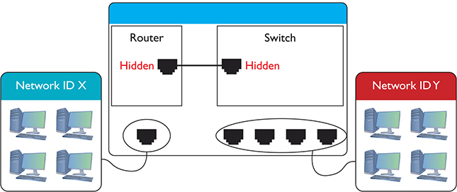
Figure 7-4  Home router diagram

Note that both boxes connect two networks. They differ in that one side of the home router connects directly to a built-in switch. That’s convenient! You don’t have to buy a separate switch to connect multiple computers to the home router.

All routers—big and small, plain or bundled with a switch—examine packets and then send the packets to the proper destination. Let’s look at that process in more detail now.

Test Specific

Routing Tables

Routing begins as packets come into the router for handling (Figure 7-5). The router immediately strips off any of the Layer 2 information and queues the resulting IP packet (Figure 7-6) based on when it arrived (unless it’s using Quality of Service [QoS], in which case it can be prioritized by a wide array of factors—Chapter 11 takes a closer look at QoS).

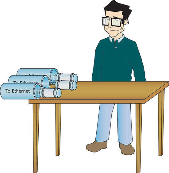
Figure 7-5  Incoming packets

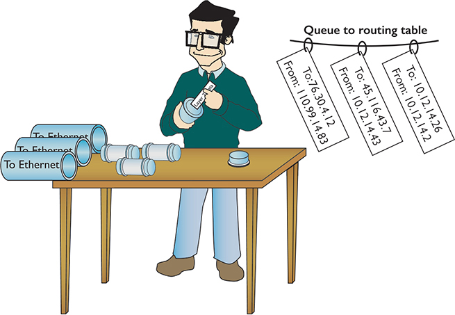
Figure 7-6  All incoming packets stripped of Layer 2 data and queued for routing

The router inspects each packet’s destination IP address and then sends the IP packet out the correct port. To perform this inspection, every router comes with a routing table that tells the router exactly where to send the packets. This table is the key to understanding and controlling the process of forwarding packets to their proper destination. Figure 7-7 shows a routing table for a typical home router. Each row in this routing table defines a single route. Each column identifies one of two specific criteria. Some columns define which packets are for the route and other columns define which port to send them out. (We’ll break these down shortly.)

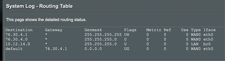
Figure 7-7  Routing table from a home router

The router in this example has only two ports internally: one port that connects to an Internet service provider, labeled as WAN0 eth0 in the Iface and Type columns of the table, and another port that connects to the router’s built-in switch, labeled LAN br0 in the table. Due to the small number of ports, this little router table has only four routes. Wait a minute: four routes and only two ports? No worries, there is not a one-to-one correlation of routes to ports, as you will soon see. Let’s inspect this routing table.

Reading Figure 7-7 from left to right shows the following:

•   Destination  A defined network ID. Every network ID directly connected to one of the router’s ports is always listed here.

•   Gateway  The IP address for the next hop router; in other words, where the packet should go. If the outgoing packet is for a network ID that’s not directly connected to the router, the Gateway column tells the router the IP address of a router to which to send this packet. That router then handles the packet, and your router is done. (Well-configured routers ensure a packet gets to where it needs to go.) If the network ID is directly connected to the router, then you don’t need a gateway. If there is no gateway needed, most routing tables put either *, 0.0.0.0, or On-link in this column.

•   Genmask  To define a network ID, you need a subnet mask (described in Chapter 6), which this router calls Genmask. (I know, I know, but I have no idea who or what decided to replace the standard term “subnet mask” with “genmask.”)

•   Flags  Describes the destination. For instance, U means that the route is up and working. H means this route is a host, or in other words, a complete IP address for a system on the network, not a subnet. G means this is the route to the gateway.

•   Metric, Ref, and Use  Most small networks are simple enough that these values (which are used for picking the best route to a destination) will all be 0. We’ll take a closer at these values in the “Routing Metrics” section.

•   Type and Iface  Tell the router which of its ports to use and what type of port it is. This router uses the Linux names for interfaces, so eth0 and br0. Other routing tables use the port’s IP address or some other description. Some routers, for example, use Gig0/0 or Gig0/1, and so on.

The router uses the combination of the destination and subnet mask (genmask, here) to see if a packet matches a route. For example, if you had a packet with the destination IP address of 10.12.14.26 coming into the router, the router would use the subnet mask to discover the network ID. It would quickly determine that the packet matches the third route shown in Figure 7-8.

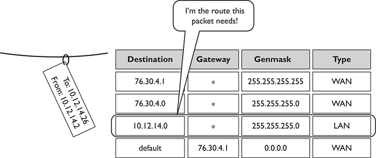
Figure 7-8  Routing table showing the route for a packet

A routing table looks like a table, so there’s an assumption that the router will start at the top of the table and march down until it finds the correct route. That’s not accurate. The router compares the destination IP address on a packet to every route listed in the routing table and only then sends the packet out. If a packet matches more than one route, the router uses the better route (we’ll discuss this more in a moment).

The most important trick to reading a routing table is to remember that a zero (0) means “anything.” For example, in Figure 7-7, the third route’s destination network ID is 10.12.14.0. You can compare that to the subnet mask (255.255.255.0) to confirm that this is a /24 network. This tells you that any value (between 1 and 254) is acceptable for the last value in the 10.12.14.0/24 network ID.

A properly configured router must have a route for any packet it might encounter. Routing tables tell you a lot about the network connections. From just this single routing table, for example, the diagram in Figure 7-9 can be drawn.

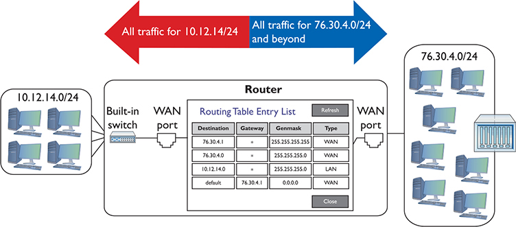
Figure 7-9  The network based on the routing table in Figure 7-7

Take another look at Figure 7-8. Notice the last route. How do I know the 76.30.4.1 port connects to another network? The fourth line of the routing table shows the default route for this router, and (almost) every router has one. In this case it’s labeled “default” so you can’t miss it. You’ll also commonly see the default destination listed as 0.0.0.0. You can interpret this line as follows:

(Any destination address) (with any subnet mask) (forward it to 76.30.4.1) (using my WAN port)

The default route is very important because this tells the router exactly what to do with every incoming packet unless another line in the routing table gives another route. Excellent! Interpret the other lines of the routing table in Figure 7-7 in the same fashion:

(Any packet for the 10.12.14.0) (/24 network ID) (don’t use a gateway) (just ARP on the LAN interface to get the MAC address and send it directly to the recipient)

(Any packet for the 76.30.4.0) (/24 network ID) (don’t use a gateway) (just ARP on the WAN interface to get the MAC address and send it directly to the recipient)

I’ll let you in on a little secret. Routers aren’t the only devices that use routing tables. In fact, every node (computer, printer, TCP/IP-capable soda dispenser, whatever) on the network also has a routing table. The main difference is that these routing tables also include rules for routing broadcast and multicast packets.

At first, this may seem silly—doesn’t every computer have a single connection that all traffic has to flow through? Every packet sent out of your computer uses the routing table to figure out where the packet should go, whether directly to a node on your network or to your gateway. Here’s an example of a routing table in Windows. This machine connects to the home router described earlier, so you’ll recognize the IP addresses it uses. (The results screen of the route print command is very long, even on a basic system, so I’ve deleted a few parts of the output for the sake of brevity.)

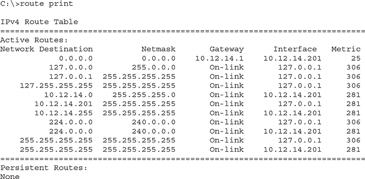
Unlike the routing table for the typical home router you saw in Figure 7-7, this one seems a bit more complicated. My PC has only a single NIC, though, so it’s not quite as complicated as it might seem at first glance.

Take a look at the details. First note that my computer has an IP address of 10.12.14.201/24 and 10.12.14.1 as the default gateway. The interface entries have actual IP addresses—10.12.14.201, plus the loopback of 127.0.0.1—instead of the word “LAN.” Second—and this is part of the magic of routing—is something called the metric.

A metric is a relative value that defines the desirability of a route. Routers often know more than one route to get a packet to its destination. If a route suddenly goes down, then the router could use an alternative route to deliver a packet. Figure 7-10 shows a networked router with two routes to the same network: a route to Network B with a metric of 1 using Route 1, and a second route to Network B using Route 2 with a metric of 10.

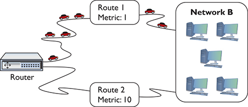
Figure 7-10  Two routes to the same network

The route with the lowest metric always wins. In this case, the router will always use the route with the metric of 1, unless that route suddenly stopped working. In that case, the router would automatically switch to the route with the 10 metric (Figure 7-11). This is how the Internet works! The entire Internet is nothing more than a whole bunch of big, powerful routers connected to lots of other big, powerful routers. Connections go up and down all the time, and routers (with multiple routes) constantly talk to each other, detecting when a connection goes down and automatically switching to alternate routes.

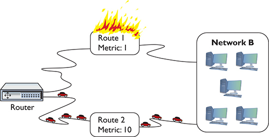
Figure 7-11  When a route no longer works, the router automatically switches.

I’ll go through this routing table one line at a time. Every address is compared to every line in the routing table before the packet goes out, so it’s no big deal if the default route is at the beginning or the end of the table.

The top line defines the default route: (Any destination address) (with any subnet mask) (forward it to my default gateway) (using my NIC) (Metric of 25 to use this route). Anything that’s not local goes to the router and from there out to the destination (with the help of other routers).

The next three lines tell your system how to handle the loopback address. The second line is straightforward, but examine the first and third lines carefully. Earlier you learned that only 127.0.0.1 is the loopback, and according to the first route, any packet with a network ID of 127.0.0.0/8 will be sent to the loopback. The third line handles the broadcast traffic for the loopback.

The next line defines the local connection: (Any packet for the 10.12.14.0) (/24 network ID) (don’t use a gateway) (just ARP on the LAN interface to get the MAC address and send it directly to the recipient) (Metric of 1 to use this route).

Okay, on to the next line. This one’s easy. Anything addressed to this machine should go right back to it through the loopback (127.0.0.1).

The next line, a directed broadcast, is for broadcasting to the other computers on the same network ID (in rare cases, you could have more than one network ID on the same LAN).

The next two lines are for the multicast address range. Windows and macOS put these lines in automatically.

The bottom lines each define a limited broadcast.

When you send a limited broadcast (255.255.255.255), it will reach every node on the local network—even nodes with differing network IDs.

Try This!

Just for fun, let’s add one more routing table; this time from my Ubiquiti EdgeMax router, which is doing a great job of connecting me to the Internet! I access the EdgeMax router remotely from my system using SSH, log in, and then run this command:

show ip route

Don’t let all the output shown next confuse you. The first part, labeled Codes, is just a legend to let you know what the letters at the beginning of each row mean.

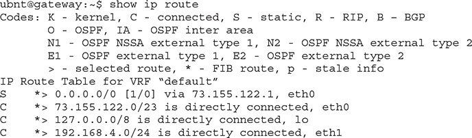
These last four lines are the routing table. The router has two active Ethernet interfaces called eth0 and eth1. This is how the EdgeMax (which is based on Linux) names Ethernet interfaces.

Reading from the bottom, you see that eth1 is directly connected (the C at the beginning of the line—and it explicitly reveals this as well) to the network 192.168.4.0/24. Any packets that match 192.168.4.0/24 go out on eth1. Next line up, you can see the entry for the loopback device, lo, taking all packets matching 127.0.0.0/8. Second from the top, any packets for the connected 73.155.122.0/23 network go out on eth0. Finally, the top route gets an S for static because it was manually set, not inserted by a routing protocol like OSPF. This is the default route because its route is 0.0.0.0/0.

In this section, you’ve seen three different types of routing tables from three different types of devices. Even though these routing tables have different ways to list the routes and different ways to show the categories, they all perform the same job: moving IP packets to the correct interface to ensure they get to where they need to go.

Freedom from Layer 2

Routers enable you to connect different types of network technologies. You now know that routers strip off all of the Layer 2 data from the incoming packets, but thus far you’ve only seen routers that connect to different Ethernet networks—and that’s just fine with routers. But routers can connect to almost anything that stores IP packets. Not to take away from some very exciting upcoming chapters, but Ethernet is not the only networking technology out there. Once you want to start making long-distance connections, Ethernet is not the only choice, and technologies with names like Data-Over-Cable Service Interface Specification (DOCSIS) (for cable modems) or passive optical network (PON) (for fiber to the premises) enter the mix. These technologies are not Ethernet, and they all work very differently than Ethernet. The only common feature of these technologies is they all carry IP packets inside their Layer 2 encapsulations.

Most enterprise (that is, not home) routers enable you to add interfaces. You buy the router and then snap in different types of interfaces depending on your needs. Note the Cisco router in Figure 7-12. Like many Cisco routers, you can buy and add removable modules. If you want to connect to an LTE (cellular phone) network, you buy an LTE module.

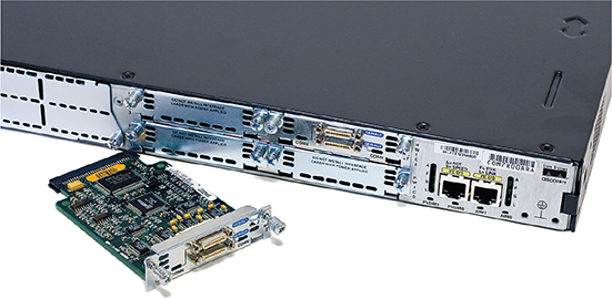
Figure 7-12  Modular Cisco router

Network Address Translation

Many regions of the world have depleted their available IPv4 addresses already and the end for everywhere else is in sight. Although you can still get an IP address from an Internet service provider (ISP), the days of easy availability are over. Routers running some form of network address translation (NAT) hide the IP addresses of computers on the LAN but still enable those computers to communicate with the broader Internet. NAT extended the useful life of IPv4 addressing on the Internet for many years. NAT is extremely common and heavily in use, so learning how it works is important. Note that many routers offer NAT as a feature in addition to the core capability of routing. NAT is not routing, but a separate technology. With that said, you are ready to dive into how NAT works to protect computers connected by router technology and conserve IP addresses as well.

The Setup

Here’s the situation. You have a LAN with five computers that need access to the Internet. With classic TCP/IP and routing, several things have to happen. First, you need to get a block of legitimate, unique, expensive IP addresses from an ISP. You could call up an ISP and purchase a network ID—say, 1.2.3.136/29. Second, you assign an IP address to each computer and to the LAN connection on the router. Third, you assign the IP address for the ISP’s router to the WAN connection on the local router, such as 1.2.4.1. After everything is configured, the network looks like Figure 7-13. All of the clients on the network have the same default gateway (1.2.3.137). This router, called a gateway, acts as the default gateway for a number of client computers.

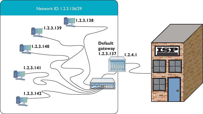
Figure 7-13  Network setup

This style of network mirrors how computers in LANs throughout the world connected to the Internet for the first 20+ years, but the major problem of a finite number of IP addresses worsened as more and more computers connected.

Port Address Translation

Most internal networks today don’t have one machine, of course. Instead, they use a block of private IP addresses for the hosts inside the network. They connect to the Internet through one or more public IP addresses.

The most common form of NAT that handles this one-to-many connection—called port address translation (PAT)—uses port numbers to map traffic from specific machines in the network. Let’s use a simple example to make the process clear: John has a network at his office that uses the private IP addressing space of 192.168.1.0/24. All the computers in the private network connect to the Internet through a single router using PAT with the global IP address of 208.190.121.12/24. See Figure 7-14.

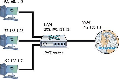
Figure 7-14  John’s network setup

When an internal machine initiates a session with an external machine, such as a Web browser accessing a Web site, the source and destination IP addresses and port numbers for the TCP segment or UDP datagram are recorded in the NAT device’s translation table, and the private IP address is swapped for the public IP address on each packet. The port number used by the internal computer for the session may also be translated into a unique port number, in which case the router records this as well. See Figure 7-15.

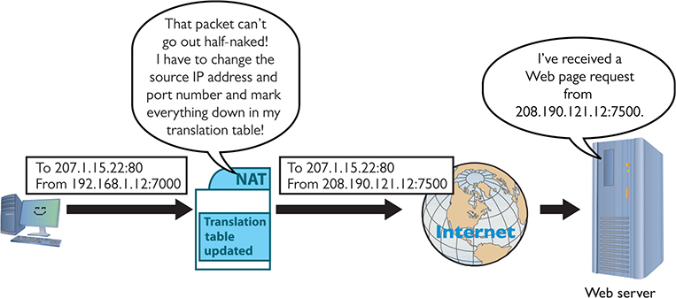
Figure 7-15  PAT in action—changing the source IP address and port number to something usable on the Internet

Table 7-1 shows a sample of the translation table inside the PAT router. Note that more than one computer translation has been recorded.

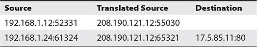
Table 7-1  Sample NAT Translation Table

When the receiving system sends the packet back, it reverses the IP addresses and ports. The router compares the incoming destination port and source IP address to the entry in the NAT translation table to determine which IP address to put back on the packet. It then sends the packet to the correct computer on the network.

This mapping of internal IP address and port number to a translated IP address and port number enables perfect tracking of packets out and in. PAT can handle many internal computers with a single public IP address because the TCP/IP port number space is big, as you’ll recall from previous chapters, with values ranging from 1 to 65535. Some of those port numbers are used for common protocols, but many tens of thousands are available for PAT to work its magic.

PAT takes care of many of the problems facing IPv4 networks exposed to the Internet. You don’t have to use legitimate Internet IP addresses on the LAN, and the IP addresses of the computers behind the routers are somewhat isolated (but not safe) from the outside world.

Since the router is revising the packets and recording the IP address and port information already, why not enable it to handle ports more aggressively? Enter port forwarding, stage left.

Port Forwarding

The obvious drawback to relying exclusively on PAT for network address translation is that it only works for outgoing communication, not incoming communication. For traffic originating outside the network to access an internal machine, such as a Web server hosted inside your network, you need to use other technologies.

Static NAT (SNAT) maps a single routable (that is, not private) IP address to a single machine, enabling you to access that machine from outside the network and vice versa. The NAT router keeps track of the IP address or addresses and applies them permanently on a one-to-one basis with computers on the network. With port forwarding, you can designate a specific local address for various network services. Computers outside the network can request a service using the public IP address of the router and the port number of the desired service. The port-forwarding router would examine the packet, look at the list of services mapped to local addresses, and then send that packet along to the proper recipient.

If you’d like users outside of your network to have access to an internal Web server, for example, you can set up a port forwarding rule for it. The router in Figure 7-16 is configured to forward all port 8080 packets to an internal Web server at port 80.

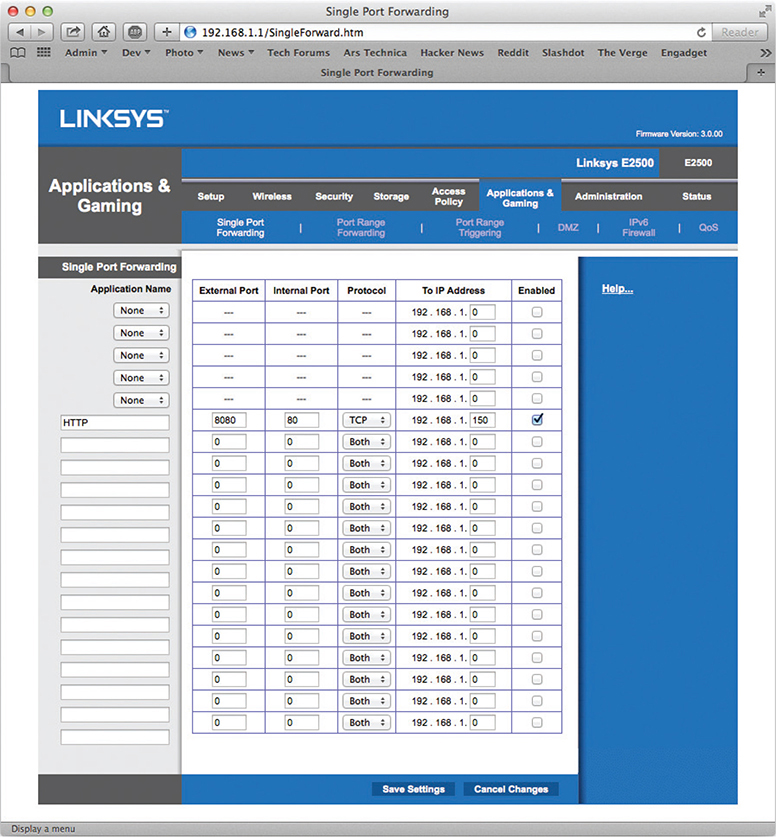
Figure 7-16  Setting up port forwarding on a home router

To access that internal Web site from outside your local network, you would have to change the URL in the Web browser by specifying the port request number. Figure 7-17 shows a browser that has :5000 appended to the URL, which tells the browser to make the HTTP request to port 5000 rather than port 80.

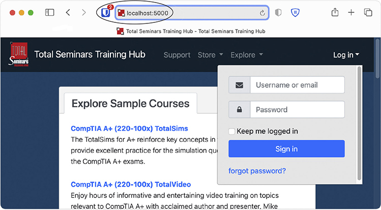
Figure 7-17  Changing the URL to access a Web site using a nondefault port number

Configuring NAT

Configuring NAT on home routers is a no-brainer as these boxes invariably have NAT turned on automatically. Figure 7-18 shows the screen on my home router for NAT. Note the radio buttons that say Gateway and Router.

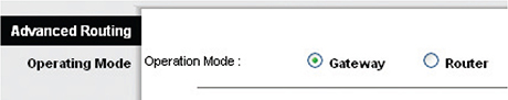
Figure 7-18  NAT setup on home router

By default, the router is set to Gateway, which is Linksys-speak for “NAT is turned on.” If I wanted to turn off NAT, I would set the radio button to Router.

Figure 7-19 shows a router configuration screen on a Cisco router. Commercial routers enable you to do a lot more with NAT.

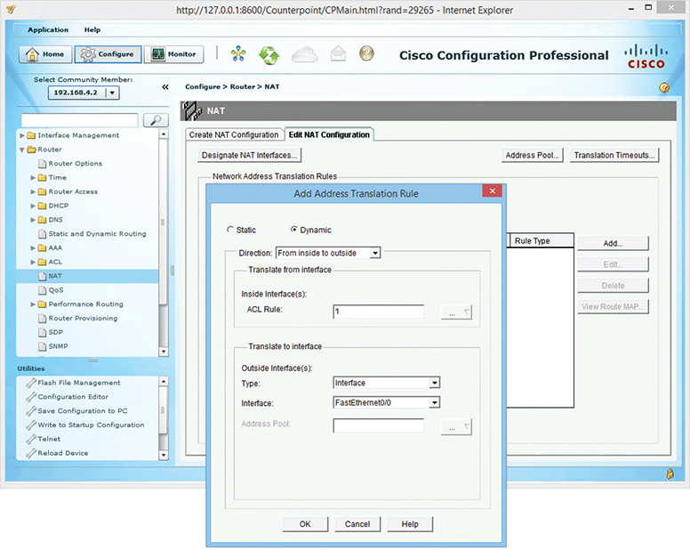
Figure 7-19  Configuring NAT on a commercial-grade router

Dynamic Routing

Based on what you’ve read up to this point, it would seem that routes in your routing tables come from two sources: either they are manually entered or they are detected at setup by the router. In either case, a route seems static, just sitting there and never changing. And based on what you’ve seen so far, that’s true. Routers can have static routes—routes that do not change. But most routers also have the capability to update their routes dynamically with dynamic routing protocols (both IPv4 and IPv6). Dynamic routing is a process that routers use to update routes to accommodate conditions, such as when a line goes down because of an electrical blackout. Dynamic routing protocols enable routers to work around such problems.

Dynamic routing protocols really shine when you manage a complex network. What if your routers look like Figure 7-20? Do you really want to try to set up all these routes statically? What happens when something changes? Can you imagine the administrative nightmare?

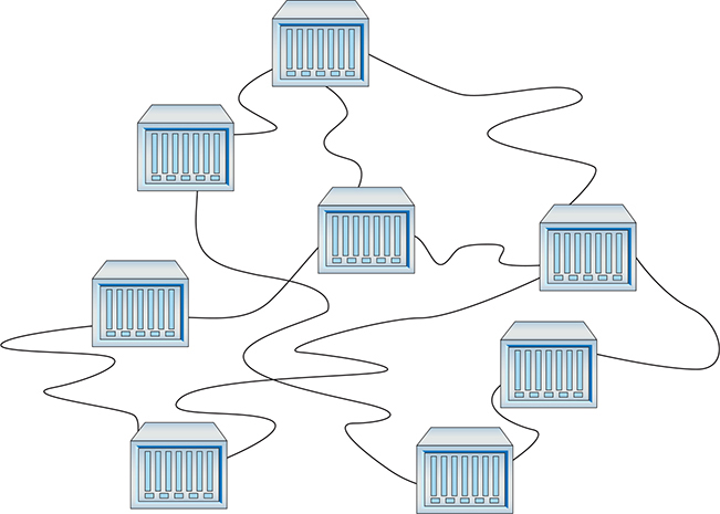
Figure 7-20  Lots of routers

Dynamic routing protocols give routers the capability to talk to each other so they know what’s happening, not only to the other directly connected routers, but also to routers two or more hops away. Each network/router a packet passes through is a hop.

CompTIA Network+ competencies break the many types of routing protocols into three distinct groups: distance vector, link state, and hybrid. CompTIA obsesses over these different types of routing protocols, so this chapter does too!

Routing Metrics

Earlier in the chapter, you learned that routing tables contain a factor called a metric. A metric is a relative value that routers use when they have more than one route to get to another network. Unlike the gateway routers in our homes, a more serious router often has multiple connections to get to a particular network. This is the beauty of routers combined with dynamic protocols. If a router suddenly loses a connection, it has alternative routes to the same network. It’s the role of the metric setting for the router to decide which route to use.

There is no single rule to set the metric value in a routing table. The various types of dynamic protocols use different criteria. Here are some common criteria for determining a metric.

•   Hop count  The hop count is a fundamental metric value for the number of routers a packet will pass through on the way to its destination network. For example, if Router A needs to go through three intermediate routers to reach a network connected to Router C, the hop count is 3. The hop occurs when the packet is handed off to each subsequent router. (I’ll go a lot more into hops and hop count in “Distance Vector and Path Vector,” next.)

•   Bandwidth  Some connections handle more data than others. An ancient 10BASE-T interface tops out at 10 Mbps. A 40GBASE-LR4 interface flies along at up to 40 Gbps.

•   Delay  Say you have a race car that has a top speed of 200 miles per hour, but it takes 25 minutes to start the car. If you press the gas pedal, it takes 15 seconds to start accelerating. If the engine runs for more than 20 minutes, the car won’t go faster than 50 miles per hour. These issues prevent the car from doing what it should be able to do: go 200 miles per hour. Delay is like that. Hundreds of issues occur that slow down network connections between routers. These issues are known collectively as latency. A great example is a cross-country fiber connection. The distance between New York and Chicago causes a delay that has nothing to do with the bandwidth of the connection.

•   Cost  Some routing protocols use cost as a metric for the desirability of that particular route. A route through a low-bandwidth connection, for example, would have a higher cost value than a route through a high-bandwidth connection. A network administrator can also manually add cost to routes to change the route selection.

Different dynamic routing protocols use one or more of these criteria to calculate their own routing metric. As you learn about these protocols, you will see how each of these calculates its own metrics differently.

Distance Vector and Path Vector

Distance vector routing protocols were the first to appear in TCP/IP routing. The cornerstone of all distance vector routing protocols is the metric. The simplest metric sums the hops (the hop count) between a router and a network, so if you had a router one hop away from a network, the metric for that route would be 1; if it were two hops away, the metric would be 2.

All network connections are not equal. A router might have two one-hop routes to a network—one using a fast connection and the other using a slow connection. Administrators set the metric of the routes in the routing table to reflect the speed. The slow single-hop route, for example, might be given the metric of 10 rather than the default of 1 to reflect the fact that it’s slow. The total metric for this one-hop route is 10, even though it’s only one hop. Don’t assume a one-hop route always has a metric of 1.

Distance vector routing protocols calculate the metric number to get to a particular network ID and compare that metric to the metrics of all the other routes to get to that same network ID. The router then chooses the route with the lowest metric.

For this to work, routers using a distance vector routing protocol transfer their entire routing table to other routers in the WAN. Each distance vector routing protocol has a maximum number of hops that a router will send its routing table to keep traffic down.

Assume you have four routers connected as shown in Figure 7-21. All of the routers have routes set up between each other with the metrics shown. You add two new networks, one that connects to Router A and the other to Router D. For simplicity, call them Network ID X and Network ID Y. A computer on one network wants to send packets to a computer on the other network, but the routers in between Routers A and D don’t yet know the two new network IDs. That’s when distance vector routing protocols work their magic.

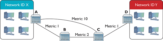
Figure 7-21  Getting a packet from Network ID X to Network ID Y? No clue!

Because all of the routers use a distance vector routing protocol, the problem gets solved quickly. At a certain defined time interval (usually 30 seconds or less), the routers begin sending each other their routing tables (the routers each send their entire routing table, but for simplicity just concentrate on the two network IDs in question). On the first iteration, Router A sends its route to Network ID X to Routers B and C. Router D sends its route to Network ID Y to Router C (Figure 7-22).

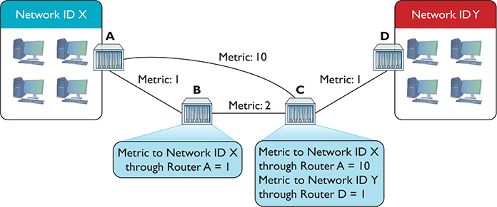
Figure 7-22  Routes updated

This is great—Routers B and C now know how to get to Network ID X, and Router C can get to Network ID Y. There’s still no complete path, however, between Network ID X and Network ID Y. That’s going to take another interval. After another set amount of time, the routers again send their now updated routing tables to each other, as shown in Figure 7-23.

Figure 7-23  Updated routing tables

Router A knows a path now to Network ID Y, and Router D knows a path to Network ID X. As a side effect, Router B and Router C have two routes to Network ID X. Router B can get to Network ID X through Router A and through Router C. Similarly, Router C can get to Network ID X through Router A and through Router B. What to do? In cases where the router discovers multiple routes to the same network ID, the distance vector routing protocol deletes all but the route with the lowest metric (Figure 7-24).

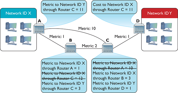
Figure 7-24  Deleting routes with higher metrics

On the next iteration, Routers A and D get updated information about the lower metric to connect to Network IDs X and Y (Figure 7-25).

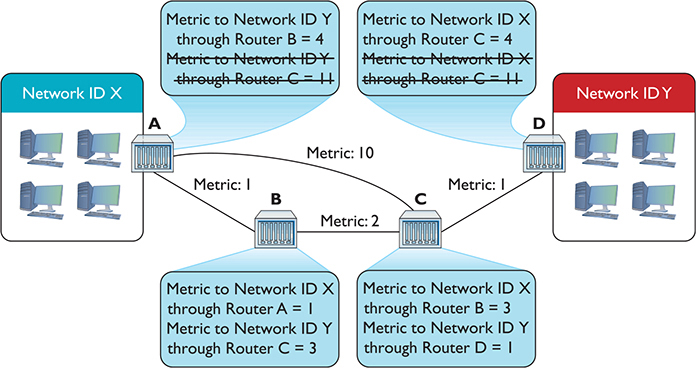
Figure 7-25  Argh! Multiple routes!

Just as Routers B and C only kept the routes with the lowest metrics, Routers A and D keep only the lowest-metric routes to the networks (Figure 7-26).

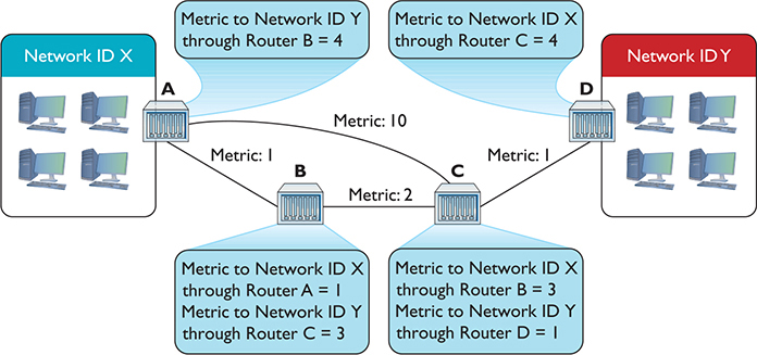
Figure 7-26  Last iteration

Now Routers A and D have a lower-metric route to Network IDs X and Y. They’ve removed the higher-metric routes and begin sending data.

At this point, if routers were human they’d realize that each router has all the information about the network and stop sending each other routing tables. Routers using distance vector routing protocols, however, aren’t that smart. The routers continue to send their complete routing tables to each other, but because the information is the same, the routing tables don’t change.

At this point, the routers are in convergence (also called steady state), meaning the updating of the routing tables for all the routers has completed. Assuming nothing changes in terms of connections, the routing tables will not change. In this example, it takes three iterations to reach convergence.

So what happens if the route between Routers B and C breaks? The routers have deleted the higher-metric routes, only keeping the lower-metric route that goes between Routers B and C. Does this mean Router A can no longer connect to Network ID Y and Router D can no longer connect to Network ID X? Yikes! Yes, it does. At least for a while.

Routers that use distance vector routing protocols continue to send to each other their entire routing table at regular intervals. After a few iterations, Routers A and D will once again know how to reach each other, although they will connect through the once-rejected slower connection.

Distance vector routing protocols work fine in a scenario such as the previous one that has only four routers. Even if you lose a router, a few minutes later the network returns to convergence. But imagine if you had tens of thousands of routers (the Internet). Convergence could take a very long time indeed. As a result, a pure distance vector routing protocol works fine for a network with a few (less than ten) routers, but it isn’t good for large networks.

Routers can use one of two distance vector routing protocols: RIPv1 or RIPv2. Plus there’s an option to use a path vector routing protocol, BGP.

RIPv1

The granddaddy of all distance vector routing protocols is the Routing Information Protocol (RIP). The first version of RIP—called RIPv1—dates from the 1980s, although its predecessors go back all the way to the beginnings of the Internet in the 1960s. RIP (either version) has a maximum hop count of 15, so your router will not talk to another router more than 15 routers away. This plagues RIP because a routing table request can literally loop all the way around back to the initial router.

RIPv1 sent out an update every 30 seconds. This also turned into a big problem because every router on the network would send its routing table at the same time, causing huge network overloads.

As if these issues weren’t bad enough, RIPv1 didn’t know how to use variable-length subnet masking (VLSM), where networks that are connected through the router use different subnet masks. Plus, RIPv1 routers had no authentication, leaving them open to hackers sending false routing table information. RIP needed an update.

RIPv2

RIPv2, adopted in 1994, is the current version of RIP. It works the same way as RIPv1, but fixes many of the problems. RIPv2 supports VLSM, includes built-in authentication, swaps broadcasting for multicast, and increases the time between updates from 30 seconds to 90 seconds.

Most routers still support RIPv2, but RIP’s many problems, especially the time to convergence for large WANs, make it obsolete for all but small, private WANs that consist of a few routers. The increase in complexity of networks since the 1990s demanded a far more robust dynamic routing protocol. That doesn’t mean RIP rests in peace! RIP is both easy to use and simple for manufacturers to implement in their routers, so most routers, even home routers, can use RIP (Figure 7-27). If your network consists of only two, three, or four routers, RIP’s easy configuration often makes it worth putting up with slower convergence.

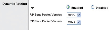
Figure 7-27  Setting RIP in a home router

BGP

The explosive growth of the Internet in the 1980s required a fundamental reorganization in the structure of the Internet itself, and one big part of this reorganization was the call to make the “big” routers use a standardized dynamic routing protocol. Implementing this was much harder than you might think because the entities that govern how the Internet works do so in a highly decentralized fashion. Even the organized groups, such as the Internet Society (ISOC), the Internet Assigned Numbers Authority (IANA), and the Internet Engineering Task Force (IETF), are made up of many individuals, companies, and government organizations from across the globe. This decentralization made the reorganization process take time and many meetings.

What came out of this process was an organizational concept called Autonomous Systems. An Autonomous System (AS) is one or more networks that share a unified “policy” regarding how they exchange traffic with other Autonomous Systems. (These policies are usually economic or political decisions made by whoever administers the AS.) Figure 7-28 illustrates the decentralized structure of the Internet.

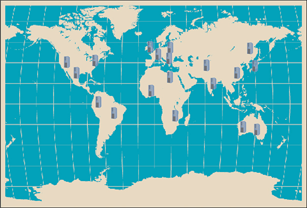
Figure 7-28  The Internet

Each Autonomous System must have a special globally unique Autonomous System Number (ASN) assigned by IANA.

Originally a 16-bit number, the current ASNs are 32 bits, displayed as two 16-bit numbers separated by a dot. So, 1.33457 would be a typical ASN. This isn’t work the computers do for us like DHCP—the routers that comprise the AS have to be configured to use the ASN assigned by IANA. See Figure 7-29.

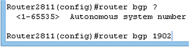
Figure 7-29  Configuring a Cisco router to use an ASN

When routers in one AS need to communicate with routers in another AS, they use an Exterior Gateway Protocol (EGP). The network or networks within an AS communicate with protocols as well: Interior Gateway Protocols (IGPs).

The easy way to keep these terms separate is to appreciate that although many protocols can be used within each Autonomous System, the Internet uses a single protocol for AS-to-AS communication: the Border Gateway Protocol (BGP). BGP is the glue of the Internet, connecting all of the Autonomous Systems. Other dynamic routing protocols such as OSPF are, by definition, IGPs. The current version of BGP is BGP-4.

Try This!

A lot of authors refer to BGP as a hybrid routing protocol, but it’s more technically a path vector routing protocol. BGP routers advertise information passed to them from different Autonomous Systems’ edge routers—that’s what the AS-to-AS routers are called.

BGP also knows how to handle a number of situations unique to the Internet. If a router advertises a new route that isn’t reliable, most BGP routers will ignore it. BGP also supports policies for limiting which and how other routers may access an ISP.

BGP implements and supports route aggregation, a way to simplify routing tables into manageable levels. Rather than trying to keep track of every router on the Internet, the backbone routers track the shortest common network ID(s) of all of the routes managed by each AS.

Route aggregation is complicated, but an analogy should make its function clear. A computer in Prague in the Czech Republic sends a packet intended to go to a computer in Chicago, Illinois, USA. When the packet hits one of the BGP routers, the router doesn’t have to know the precise location of the recipient. It knows the router for the United States and sends the packet there. The U.S. router knows the Illinois router, which knows the Chicago router, and so on.

BGP is the obvious (only) choice for edge routers, but distance vector protocols aren’t the only game in town when it comes to the inside of your network. Let’s look at another family: link state routing protocols.

Link State

The limitations of RIP motivated the demand for a faster protocol that took up less bandwidth on a WAN. The basic idea was to come up with a dynamic routing protocol that was more efficient than routers that simply sent out their entire routing table at regular intervals. Why not instead simply announce and forward individual route changes as they appeared? That is the basic idea of a link state dynamic routing protocol. There are only two link state dynamic routing protocols: OSPF and IS-IS.

OSPF

Open Shortest Path First (OSPF) is the most commonly used IGP in the world. Most large enterprises use OSPF on their internal networks. Even an AS, while still using BGP on its edge routers, will use OSPF internally because OSPF was designed from the ground up to work within a single AS. OSPF converges dramatically faster and is much more efficient than RIP. Odds are good that if you are using dynamic routing protocols, you’re using OSPF.

OSPF offers a number of improvements over RIP. OSPF-capable routers initially send out Hello packets, looking for other OSPF routers (see Figure 7-30). After two adjacent routers form a neighborship through the Hello packets, they exchange information about routers and networks through link state advertisement (LSA) packets. LSAs are sourced by each router and are flooded from router to router through each OSPF area.

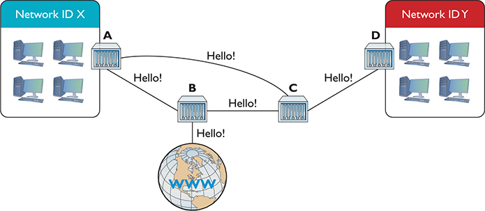
Figure 7-30  Hello!

Once all the routers communicate, they individually decide their own optimal routes, and convergence happens almost immediately. If a route goes down, OSPF routers quickly recompute a new route with stored LSAs.

OSPF’s metric is cost, which is a function of bandwidth. All possible ways to get to a destination network are computed based on cost, which is proportional to bandwidth, which is in turn proportional to the interface type (Gigabit Ethernet, 10-Gigabit Ethernet, and so on). The routers choose the lowest total cost route to a destination network.

In other words, a packet could go through more routers (hops) to get to a destination when OSPF is used instead of RIP. However, more hops doesn’t necessarily mean slower. If a packet goes through three hops where the routers are connected by fiber, for example, as opposed to a slow 1.544-Mbps link, the packet would get to its destination quicker. We make these decisions everyday as humans, too. I’d rather drive more miles on the highway to get somewhere quicker, than fewer miles on local streets where the speed limit is much lower. (Red lights and stop signs introduce driving latency as well!)

OSPF uses areas, administrative groupings of interconnected routers, to help control how routers reroute traffic if a link drops. All OSPF networks use areas, even if there is only one area. When you interconnect multiple areas, the central area—called the backbone—gets assigned the Area ID of 0 or 0.0.0.0. (Note that a single area also gets Area ID 0.) All traffic between areas has to go through the backbone.

OSPF isn’t popular by accident. It scales to large networks quite well and is supported by all but the most basic routers. By the way, did I forget to mention that OSPF also supports authentication and that the shortest-path-first method, by definition, prevents loops?

IS-IS

If you want to use a link state dynamic routing protocol and you don’t want to use OSPF, your only other option is Intermediate System to Intermediate System (IS-IS). IS-IS is extremely similar to OSPF. It uses the concept of areas and send-only updates to routing tables. IS-IS was developed at roughly the same time as OSPF and had the one major advantage of working with IPv6 from the start. IS-IS is the de facto standard for ISPs. Make sure you know that IS-IS is a link state dynamic routing protocol, and if you ever see two routers using it, call me as I’ve never seen IS-IS in action.

EIGRP

There is exactly one protocol that doesn’t really fit into either the distance vector or link state camp: Cisco’s proprietary Enhanced Interior Gateway Routing Protocol (EIGRP). Back in the days when RIP was dominant, there was a huge outcry for an improved RIP, but OSPF wasn’t yet out. Cisco, being the dominant router company in the world (a crown it still wears to this day), came out with the Interior Gateway Routing Protocol (IGRP), which was quickly replaced with EIGRP.

EIGRP has aspects of both distance vector and link state protocols, placing it uniquely into its own “hybrid” category. Cisco calls EIGRP an advanced distance vector protocol.

Dynamic Routing Makes the Internet

Without dynamic routing, the complex, self-healing Internet we all enjoy today couldn’t exist. So many routes come and go so often that manually updating static routes would be impossible. Review Table 7-2 to familiarize yourself with the differences among the different types of dynamic routing protocols.

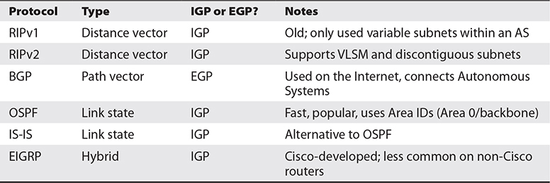
Table 7-2  Dynamic Routing Protocols

Route Redistribution and Administrative Distance

Wow, there sure are many routing protocols out there. It’s too bad they can’t talk to each other…or can they?

The routers cannot use different routing protocols to communicate with each other, but many routers can speak multiple routing protocols simultaneously. When a router takes routes it has learned by one method, say RIP or a statically set route, and announces those routes over another protocol such as OSPF, this is called route redistribution. This feature can come in handy when you have a mix of equipment and protocols in your network, such as occurs when you switch vendors or merge with another organization.

When a multilingual router has two or more protocol choices to connect to the same destination, the router uses a feature called administrative distance to determine which route is the most reliable. You’ll see this feature called route preference as well.

Working with Routers

Understanding the different ways routers work is one thing. Actually walking up to a router and making it work is a different animal altogether. This section examines practical router installation. Physical installation isn’t very complicated. With a home router, you give it power and then plug in connections. With a business-class router, you insert it into a rack, give it power, and plug in connections.

The complex part of installation comes with the specialized equipment and steps to connect to the router and configure it for your network needs. This section, therefore, focuses on the many methods and procedures used to access and configure a router.

The single biggest item to keep in mind here is that although there are many different methods for connecting, hundreds of interfaces, and probably millions of different configurations for different routers, the functions are still the same. Whether you’re using an inexpensive home router or a hyper-powerful Internet backbone router, you are always working to do one main job: connect different networks.

Connecting to Routers

When you take a new router out of the box, it’s not good for very much. You need to somehow plug into that shiny new router and start telling it what you want to do. There are a number of different methods, but one of the oldest (yet still very common) methods is to use a special serial connection. Figure 7-31 shows the classic Cisco console cable, more commonly called a rollover or Yost cable.

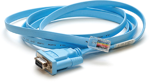
Figure 7-31  Cisco console cable

At this time, I need to make an important point: switches as well as routers often have some form of configuration interface. Granted, you have nothing to configure on a basic switch, but in later chapters, you’ll discover a number of network features that you’ll want to configure more advanced switches to use. Both routers and these advanced switches are called managed devices. In this section, I use the term router, but it’s important for you to appreciate that all routers and many better switches are all managed devices. The techniques shown here work for both!

When you first unwrap a new router, you plug the rollover cable into the console port on the router (Figure 7-32) and a serial port on a PC. If you don’t have a serial port, then buy a USB-to-serial adapter.

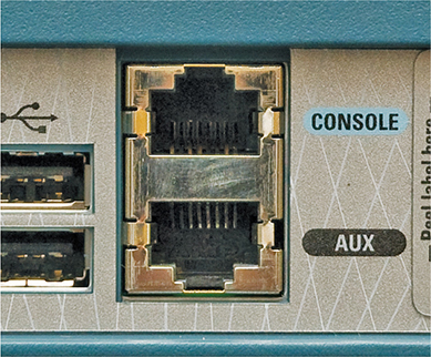
Figure 7-32  Console port

Once you’ve made this connection, you need to use a terminal emulation program to talk to the router. Two common graphical programs are PuTTY (www.chiark.greenend.org.uk/~sgtatham/putty) and HyperTerminal (www.hilgraeve.com/hyperterminal). Using these programs requires that you to know a little about serial ports, but these basic settings should get you connected:

•   9600 baud

•   8 data bits

•   1 stop bit

•   No parity

Every terminal emulator has some way for you to configure these settings. Figure 7-33 shows these settings using PuTTY.

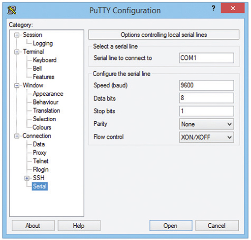
Figure 7-33  Configuring PuTTY

Now it’s time to connect. Most Cisco products run Cisco IOS, Cisco’s proprietary operating system. If you want to configure Cisco routers, you must learn IOS. Learning IOS in detail is a massive job and outside the scope of this book. No worries, because Cisco provides a series of certifications to support those who wish to become “Cisco People.” Although the CompTIA Network+ exam won’t challenge you in terms of IOS, it’s important to get a taste of how this amazing operating system works.

Once you’ve connected to the router and started a terminal emulator, you should see the initial router prompt, as shown in Figure 7-34. (If you plugged in and then started the router, you can actually watch the router boot up first.)

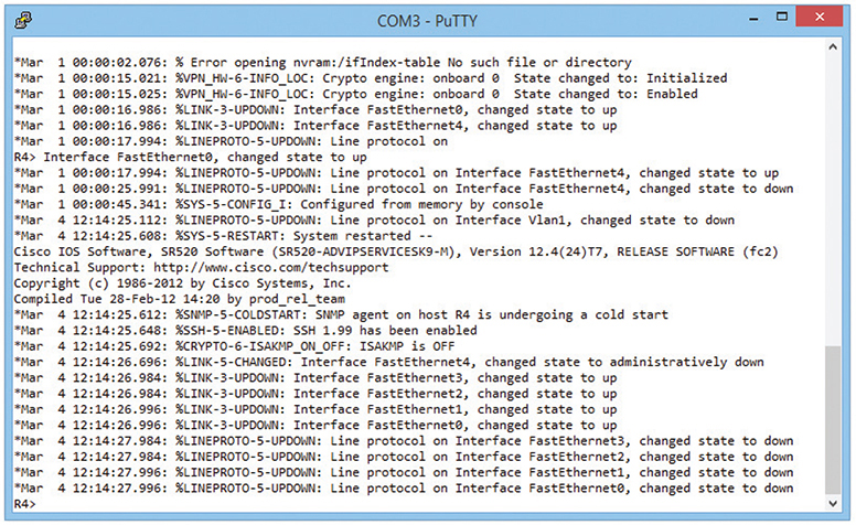
Figure 7-34  Initial router prompt

This is the IOS user mode prompt—you can’t do too much here. To get to the fun, you need to enter privileged EXEC mode. Type enable, press ENTER, and the prompt changes to

Router#

From here, IOS gets very complex. For example, the commands to set the IP address for one of the router’s ports look like this:

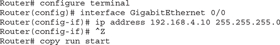
Cisco has long appreciated that initial setup is a bit of a challenge, so a brand-new router will show you the following prompt:

Simply follow the prompts, and the most basic setup is handled for you.

You will run into Cisco equipment as a network tech, and you will need to know how to use the console from time to time. For the most part, though, you’ll access a router—especially one that’s already configured—through Web access or network management software.

Web Access

Most routers come with a built-in Web interface that enables you to do everything you need on your router and is much easier to use than Cisco’s command-line IOS. For a Web interface to work, however, the router must have a built-in IP address from the factory, or you have to enable the Web interface after you’ve given the router an IP address. Bottom line? If you want to use a Web interface, you have to know the router’s IP address. If a router has a default IP address, you will find it in the documentation, as shown in Figure 7-35.

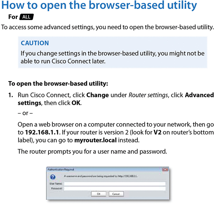
Figure 7-35  Default IP address

Never plug a new router into an existing network! There’s no telling what that router might start doing. Does it have DHCP? You might now have a rogue DHCP server. Are there routes on that router that match up to your network addresses? Then you see packets disappearing into the great bit bucket in the sky. Always fully configure your router before you place it online.

Most router people use a laptop and a crossover cable to connect to the new router. To get to the Web interface, first set a static address for your computer that will place your PC on the same network ID as the router. If, for example, the router is set to 192.168.1.1/24 from the factory, set your computer’s IP address to 192.168.1.2/24. Then connect to the router (some routers tell you exactly where to connect, so read the documentation first), and check the link lights to verify you’re properly connected. Open a Web browser and type in the IP address, as shown in Figure 7-36.

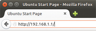
Figure 7-36  Entering the IP address

Assuming you’ve done everything correctly, you almost always need to enter a default username and password, as shown in Figure 7-37.

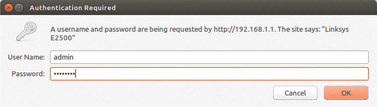
Figure 7-37  Username and password

The default username and password come with the router’s documentation. If you don’t have that information, plenty of Web sites list this data. Do a Web search on “default username password” to find one.

Once you’ve accessed the Web interface, you’re on your own to poke around to find the settings you need. There’s no standard interface—even between different versions of the same router make and model. When you encounter a new interface, take some time and inspect every tab and menu to learn about the router’s capabilities. You’ll almost always find some really cool features!

Network Management Software

The idea of a “Web-server-in-a-router” works well for single routers, but as a network grows into lots of routers, administrators need more advanced tools that describe, visualize, and configure their entire network. These tools, known as Network Management Software (NMS), know how to talk to your routers, switches, and even your computers to give you an overall view of your network. In most cases, NMS manifests as a Web site where administrators may inspect the status of the network and make adjustments as needed.

I divide NMS into two camps: proprietary tools made by the folks who make managed devices, original equipment manufacturers (OEMs), and third-party tools. OEM tools are generally very powerful and easy to use, but only work on that OEM’s devices. Figure 7-38 shows an example of Cisco Network Assistant, one of Cisco’s NMS applications. Others include the Cisco Configuration Professional and Cisco Prime Infrastructure, an enterprise-level tool.

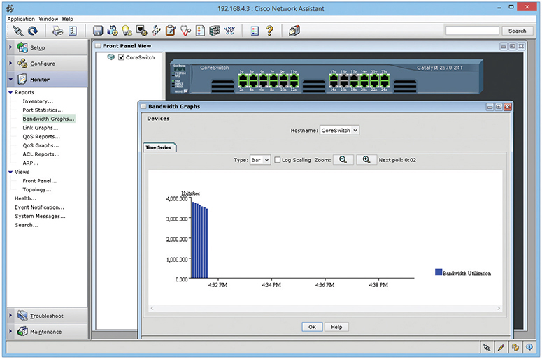
Figure 7-38  Cisco Network Assistant

A number of third-party NMS tools are out there as well; you can even find some pretty good freeware NMS options. These tools are invariably harder to configure and must constantly be updated to try to work with as many devices as possible. They usually lack the amount of detail you see with OEM NMS and lack interactive graphical user interfaces. For example, various Cisco products enable you to change the IP address of a port, whereas third-party tools only let you see the current IP settings for that port. Figure 7-39 shows OpenNMS, a popular open source NMS.

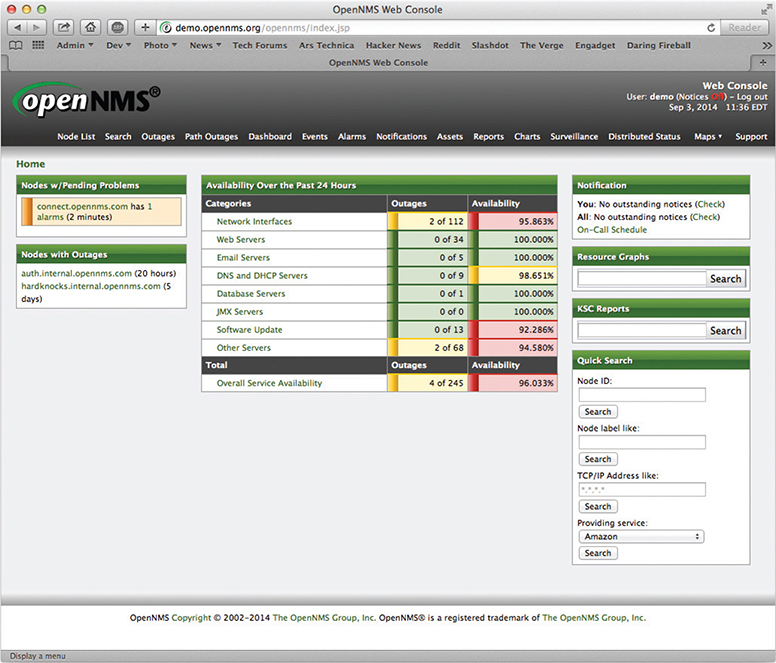
Figure 7-39  OpenNMS

Unfortunately, no single NMS tool works perfectly. Network administrators are constantly playing with this or that NMS tool in an attempt to give themselves some kind of overall picture of their networks.

Other Connection Methods

Be aware that most routers have even more ways to connect. More powerful routers may enable you to connect using the ancient Telnet protocol or its newer and safer equivalent Secure Shell (SSH). These are terminal emulation protocols that look exactly like the terminal emulators seen earlier in this chapter but use the network instead of a serial cable to connect (see Chapter 8 for details on these protocols).

Basic Router Configuration

A router, by definition, must have at least two connections. When you set up a router, you must configure every port on the router properly to talk to its connected network IDs, and you must make sure the routing table sends packets to where you want them to go. As a demonstration, Figure 7-40 uses an incredibly common setup: a single gateway router used in a home or small office that’s connected to an ISP.

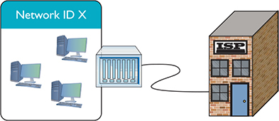
Figure 7-40  The setup

Step 1: Set Up the WAN Side

To start, you need to know the network IDs for each side of your router. The WAN side invariably connects to an ISP, so you need to know what the ISP wants you to do. If you bought a static IP address, type it in now. However—brace yourself for a crazy fact—most home Internet connections use DHCP! That’s right, DHCP isn’t just for your PC. You can set up your router’s WAN connection to use it too. DHCP is by far the most common connection to use for home routers. Access your router and locate the WAN connection setup. Figure 7-41 shows the setup for my home router set to DHCP.

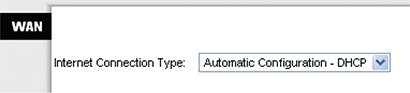
Figure 7-41  WAN router setup

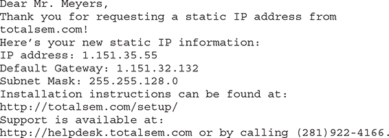
But what if I called my ISP and bought a single static IP address? This is rarely done anymore, but virtually every ISP will gladly sell you one (although you will pay three to four times as much for the connection). If you use a static IP address, your ISP will tell you what to enter, usually in the form of an e-mail message like the following:

In such a case, I would need to change the router setting to Static IP (Figure 7-42). Note how changing the drop-down menu to Static IP enables me to enter the information needed.

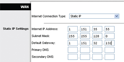
Figure 7-42  Entering a static IP

Once you’ve set up the WAN side, it’s time to head over to set up the LAN side of the router.

Step 2: Set Up the LAN Side

Unlike the WAN side, you usually have total control on the LAN side of the router. You need to choose a network ID, almost always some arbitrarily chosen private range unless you do not want to use NAT. This is why so many home networks have network IDs of 192.168.1.0/24, 192.168.2.0/24, and so forth. Once you decide on your LAN-side network ID, you need to assign the correct IP information to the LAN-side NIC. Figure 7-43 shows the configuration for a LAN NIC on my home router.

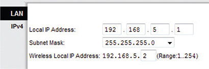
Figure 7-43  Setting up an IP address for the LAN side

Step 3: Establish Routes

Most routers are pretty smart and use the information you provided for the two interfaces to build a routing table automatically. If you need to add more routes, every router provides some method to add routes. The following shows the command entered on a Cisco router to add a route to one of its Ethernet interfaces. The term “gig0/0” is how Cisco describes Ethernet NICs in its device software. It is short for GigabitEthernet, which you may remember as being the common name (when you add a space) for 1000BaseT.

ip route 192.168.100.0 255.255.255.0 gig0/0 192.168.1.10

Step 4 (Optional): Configure a Dynamic Protocol

The rules for using any dynamic routing protocol are fairly straightforward. First, dynamic routing protocols are tied to individual interfaces, not the entire router. Second, when you connect two routers together, make sure those two interfaces are configured to use the same dynamic routing protocol. Third, unless you’re in charge of two or more routers, you’re probably not going to use any dynamic routing protocol.

The amazing part of a dynamic routing protocol is how easy it is to set up. In most cases you just figure out how to turn it on and that’s about it. It just starts working.

Step 5: Document and Back Up

Once you’ve configured your routes, take some time to document what you’ve done. A good router works for years without interaction, so by that time in the future when it goes down, odds are good you will have forgotten why you added the routes. Last, take some time to back up the configuration. If a router goes down, it will most likely forget everything and you’ll need to set it up all over again. Every router has some method to back up the configuration, however, so you can restore it later.

Router Problems

The CompTIA Network+ exam will challenge you on some basic router problems. All of these questions should be straightforward for you as long as you do the following:

•   Consider other issues first because routers don’t fail very often.

•   Keep in mind what your router is supposed to do.

•   Know how to use a few basic tools that can help you check the router.

Any router problem starts with someone not connecting to someone else. Even a small network has a number of NICs, computers, switches, and routers between you and whatever it is you’re not connecting to. Compared to most of these, a router is a pretty robust device and shouldn’t be considered as the problem until you’ve checked out just about everything else first.

In their most basic forms, routers route traffic. Yet you’ve seen in this chapter that routers can do more than just plain routing—for example, NAT. As this book progresses, you’ll find that the typical router often handles a large number of duties beyond just routing. Know what your router is doing and appreciate that you may find yourself checking a router for problems that don’t really have anything to do with routing at all.

Routing Tables and Missing Routes

Be aware that routers have some serious but rare potential problems. One place to watch is your routing table. For the most part, today’s routers automatically generate directly connected routes, and dynamic routing takes care of itself, leaving one type of route as a possible suspect: the static routes. This is the place to look when packets aren’t getting to the places you expect them to go. Look at the following sample static route:

No incoming packets for the network ID are getting out on interface 22.46.132.11. Can you see why? Yup, the Netmask is set to 255.255.255.255, and there are no computers that have exactly the address 22.46.132.0. Entering the wrong network destination, subnet mask, gateway, and so on, is very easy. If a new static route isn’t getting the packets moved, first assume you made a typo.

Make sure to watch out for missing routes. These usually take place either because you’ve forgotten to add them (if you’re entering static routes) or, more commonly, there is a convergence problem in the dynamic routing protocols. For the CompTIA Network+ exam, be ready to inspect a routing table to recognize these problems.

MTUs and PDUs

The developers of TCP/IP assumed that traffic would move over various networking technologies and packet size would vary. Each technology has a maximum size of a single protocol data unit (PDU) that can transmit, called the maximum transmission unit (MTU). The PDU for TCP at Layer 4, for example, is a segment that gets encapsulated into an IP packet (the PDU for Layer 3). The IP packet in turn gets encapsulated in some medium at Layer 2. Ethernet frames encapsulate IP packets, for example.

At each layer of encapsulation, other information gets added (such as source and destination IP or MAC address) and the PDU for that layer gets larger. Going from one network technology to another can cause a packet or frame to exceed the MTU for the receiving system, which is not a big deal. The network components know to split the packet or frame into two or more pieces to get below the MTU threshold for the next hop. The problem is that this fragmentation can increase the number of packets or frames needed to move data between two points—gross inefficiency.

Path MTU describes the largest packet size transmissible without fragmentation through all the hops in a route. Devices can use Path MTU Discovery to determine the path MTU, that maximum size. MTU size can be adjusted at the source to eliminate fragmentation.

Tools

When it comes to tools, networking comes with so many utilities and magic devices that it staggers the imagination. You’ve already seen some, like good old ping and route, but let’s add two more tools: traceroute and mtr.

The traceroute tool, as its name implies, records the route between any two hosts on a network. On the surface, traceroute is something like ping in that it sends a single packet to another host, but as it progresses, it returns information about every router between them.

Every operating system comes with traceroute, but the actual command varies among them. In Windows, the command is tracert and looks like this (I’m running a traceroute to the router connected to my router—a short trip):

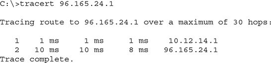
The macOS/UNIX/Linux command is traceroute and looks like this:

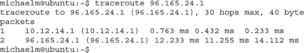
The traceroute tool is handy, not so much for what it tells you when everything’s working well, but for what it tells you when things are not working. Look at the following:

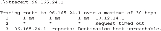
If this traceroute worked in the past but now no longer works, you know that something is wrong between your router and the next router upstream. You don’t know what’s wrong exactly. The connection may be down; the router may not be working; but at least traceroute gives you an idea where to look for the problem and where not to look.

My traceroute (mtr) is very similar to traceroute, but it’s dynamic, continually updating the route that you’ve selected (Figure 7-44). You won’t find mtr in Windows; mtr is a Linux tool. Instead, Windows users can use pathping. This utility pings each node on the route just like mtr, but instead of showing the results of each ping in real time, the pathping utility computes the performance over a set time and then shows you the summary after it has finished.

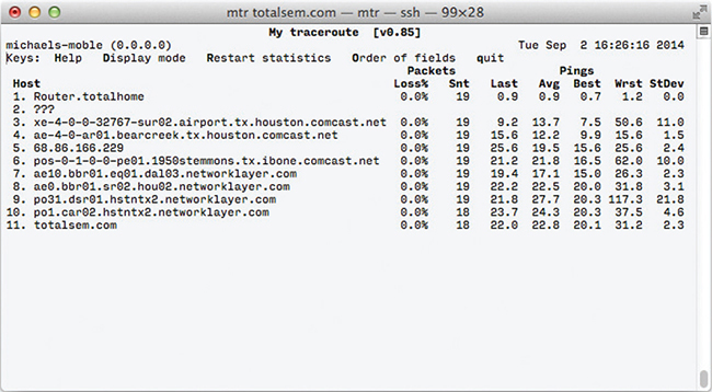
Figure 7-44  mtr in action

Packets used by tools like traceroute and mtr have a default number of hops they’ll go before being discarded by a router. At every hop, a router decreases the time to live (TTL) number in a packet until the packet reaches its destination or hits zero. This stops packets from going on forever. The final router will discard the packet and send an ICMP message to the original sender.

Each tool for doing tracing (and that includes ping and pathping) enables you to set the maximum hop count; most default at 30, as you can see in the various “over a maximum of 30 hops” notes in the screen outputs above. To set a tracert to go for many hops, for example, you’d use the -h switch and a number, like in Figure 7-45.

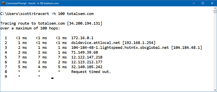
Figure 7-45  Adjusting TTL in tracert

Chapter Review

Questions

1.   What is a router?

A.   A piece of hardware that forwards packets based on IP address

B.   A device that separates your computers from the Internet

C.   A piece of hardware that distributes a single Internet connection to multiple computers

D.   A synonym for a firewall

2.   Routers must use the same type of connection for all routes, such as Ethernet to Ethernet or DOCSIS to DOCSIS.

A.   True

B.   False

3.   What technology allows you to share a single public IP address with many computers?

A.   Static address translation

B.   Natural address translation

C.   Computed public address translation

D.   Port address translation

4.   Given the following routing table:

where would a packet with the address 64.165.5.34 be sent?

A.   To the default gateway on interface WAN.

B.   To the 10.11.12.0/24 network on interface LAN.

C.   To the 64.165.5.0/24 network on interface WAN.

D.   Nowhere; the routing table does not have a route for that address.

5.   Which of the following is an EGP?

A.   BGP

B.   IGP

C.   EIGRP

D.   IS-IS

6.   What dynamic routing protocol uses link state advertisements to exchange information about networks?

A.   BGP

B.   OSPF

C.   EIGRP

D.   IS-IS

7.   What is Area 0 called in OSPF?

A.   Local Area

B.   Primary Zone

C.   Trunk

D.   Backbone

8.   Which of the following is not a name for a serial cable that you use to configure a router?

A.   Console cable

B.   Yost cable

C.   Rollover cable

D.   Null modem cable

9.   When you are first setting up a new router, you should never plug it into an existing network.

A.   True

B.   False

10.   The traceroute utility is useful for which purpose?

A.   Configuring routers remotely

B.   Showing the physical location of the route between you and the destination

C.   Discovering information about the routers between you and the destination address

D.   Fixing the computer’s local routing table

Answers

1.   A. A router is a piece of hardware that forwards packets based on IP address.

2.   B. False; a router can interconnect different Layer 2 technologies.

3.   D. Port address translation, commonly known as PAT, enables you to share a single public IP address with many computers.

4.   C. It would be sent to the 64.165.5.0/24 network on interface WAN.

5.   A. Border Gateway Protocol (BGP) is an exterior gateway protocol.

6.   B. Open Shortest Path First (OSPF) uses link state advertisement (LSA) packets to exchange information about networks.

7.   D. Area 0 is called the backbone area.

8.   D. The Yost cable, which was invented to standardize the serial console interface to connect to the router console port, is also known as a rollover or console cable.

9.   A. True; never plug a new router into an existing network.

10.   C. The traceroute utility is useful for discovering information about the routers between you and the destination address.