
This is possibly the most important chapter in the book. Although measures are what we're after, dimensions are the framework on which we'll build our cubes. Dimension names give us the nomenclature we'll use to break down our data, attributes will give us additional information about the members, and the members themselves provide the semantic points against which our measure data will be arrayed. Finally, well-designed dimension and attribute relationships will ensure the scalability of our cube solutions.
Before we can start designing dimensions, we have to figure out what dimensions we need. What problem are we trying to solve? In my opinion, this is a driving foundation of a successful business intelligence effort—identifying the problem domain.
Many BI initiatives start as "we need a data warehouse" without real direction. This is akin to someone standing in Madison, Wisconsin and declaring one day that she wants to visit every country. A wise traveler will then buy a bunch of maps, identify locations, and start working on solving the traveling salesman problem. It should soon become apparent that a huge amount of analysis is necessary—even more so if our traveler has never actually been on a train, airplane, or boat. In this research, the traveler will find that she needs a passport, luggage, and various supplies depending on the country she visits. She also needs visas. But wait. What visa she needs for a country depends on which border she's using to enter the country (and some borders can't be crossed!).
This is certainly a huge problem, and will take a very long time to plan out properly. However, all the time she spends planning is time she's not traveling. Meanwhile, she has bills to pay and a life to live, and because she hasn't actually gone anywhere, over time she'll just lose interest in the whole project.
Now what if, instead, our traveler decides that what she really wants to do is visit Europe, and specifically the Eiffel Tower? It's much easier to plan a short trip to Paris, find a cheap round-trip flight, book a hotel, figure out the visa situation, and so on. Soon she's on her way to Paris, enjoys her trip, and she's home again. Now she decides to visit Japan, and so does some more research—but this time the research doesn't take nearly as long, because she can build on what she learned on the last trip, and add in her personal experiences with what worked and what didn't.
My analogy is probably too thin, but hopefully will make the point. Don't try to sit down and design the be-all, end-all ultra data warehouse that will answer any question anyone could possibly ask. Instead, identify smaller business problems that can be solved with smaller cubes. Build a collection of cubes, and grow the solution iteratively. In this way, your users get value from what you've already built, and each project draws from the experience the team gained on the previous problem. With that in mind, let's look at some concepts behind dimensions that will serve our analysis, and then how we'll build them in Analysis Services.
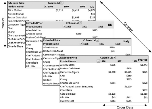
Let's look at our notional "cube" again, represented by spreadsheets. In Figure 6-1, Order Date, Country, and Product are each dimensions. Alice Mutton, Aniseed Syrup, Boston Crab Meat, and so on are members of the Product dimension. We use dimensions to organize collections of attributes into logical groupings (just as we have products, country, and time). You can see that the collection of dimensions effectively defines the collection of measures that make up our cube. In SSAS, the concept of a dimension actually exists independent of a cube. Dimensions can be the result of a single cube design, but they can also be in a database solution with no cubes. A single dimension can be used in multiple cubes, or even linked between multiple databases.
In our dimensional analysis, after identifying a problem domain, we'll have to figure out what types of questions users are likely to ask and how they will seek answers. I won't go into requirements analysis here. If you're interested in methods for gathering requirements in the data warehouse world, I recommend The Data Warehouse Lifecycle Toolkit, by Ralph Kimball, Margy Ross, Warren Thornthwaite, Joy Mundy, and Bob Becker (Wiley, 2008) or The Microsoft Data Warehouse Toolkit: With SQL Server 2005 and the Microsoft Business Intelligence Toolset by Joy Mundy and Warren Thornthwaite (Wiley, 2006). There is one big technical decision we need to make, however: do we want a star schema or a snowflake?
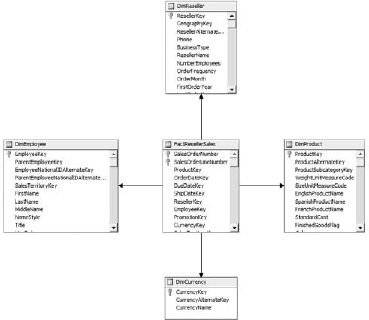
We generally have two options when creating a cube: a star or a snowflake schema. To review, a star schema has a single fact table with every dimension table linked directly to it (Figure 6-2).
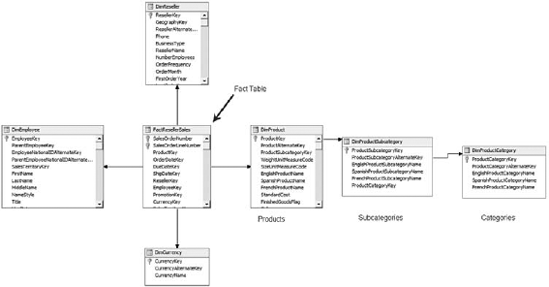
Compare this to a snowflake schema, which keeps the tables more normalized, similar to Figure 6-3.
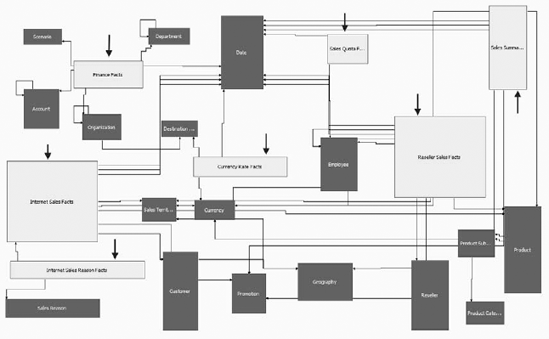
A snowflake schema will likely give way to what is often termed a multisnowflake schema, which has multiple fact tables. From here we can see a creeping problem that adds fact tables, dimension tables, supporting tables, and so on. You can see a similar result in the AdventureWorks schema in Figure 6-4, which I've annotated with arrows pointing to each fact table.
The primary advantage of a star schema is that it keeps development focused on a simple approach—one fact table, and every dimension linked to the fact table. It's important when creating a cube to keep focused on end-user usability, especially because ease of use for our analyst end user is a major reason we're building these cubes in the first place.
As an example of how a complex schema can defeat end-user usability, consider the pick list for measures and dimensions we see if we open the AdventureWorks cube in Excel (Figure 6-5).
Perhaps our analyst wants to examine the effectiveness of an ad campaign on in-store buyers based on their geographic region. So it seems logical to examine reseller sales by customer location, right? Let's continue down that path. My argument will be easier to follow if you build the report yourself. So let's build a quick Excel report in Exercise 6-1.
Note
You'll need the AdventureWorks 2008 demo cube installed and processed for this exercise. See Appendix A.
Build an Excel Report
The following steps walk you through building a report to examine reseller sales by customer location, based on the schema in Figure 6-4, and on the measures and dimensions highlighted in Figure 6-5. As you develop the report, you'll see how the complexity of the schema works against you.
Open Excel 2007.
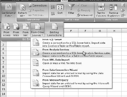
Click the Data tab. On the Data tab, click the Get External Data button, then From Other Sources, and finally From Analysis Services (Figure 6-6).
On the first page of the Data Connection Wizard, enter the server name (localhost will do if you have a single dev machine). Then click the Next button.
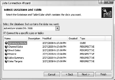
Select Adventure Works DW 2008 from the database drop-down list, and Adventure Works in the specific cube selector (Figure 6-7).
Click Next and then click Finish.
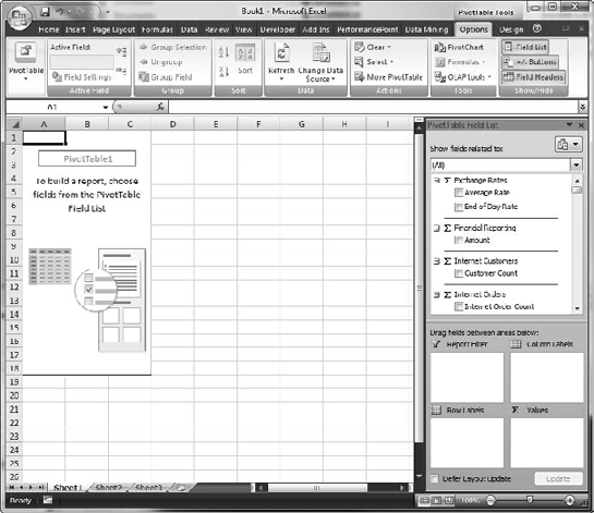
In the Import Data dialog box, select PivotTable Report and then click the OK button. You'll get a pivot table area and the PivotTable Field List (Figure 6-8).
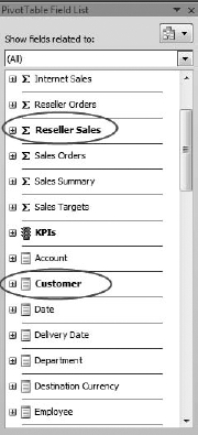
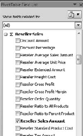
In the field list on the right, scroll down to Reseller Sales and select the Reseller Sales Amount check box (Figure 6-9).
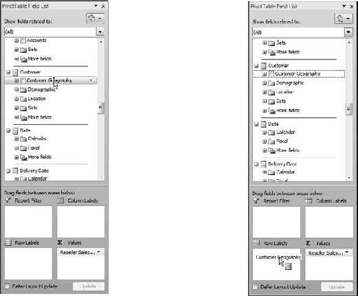
Now scroll down to Customer and drag Customer Geography to Row Labels (Figure 6-10).
When you're finished, you should have an area in the Excel spreadsheet that looks like Figure 6-11.
Click the [+] icons next to the countries to look at the region values. What happened? Read on.
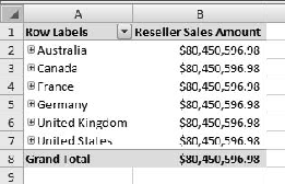
Well, it's a safe bet that those six countries didn't sell exactly the same amount of product (down to the penny), so it looks like our Customer Geography dimension isn't splitting the measure data. Why is this? A little examination of the cube structure will show us why. First we note from the pivot table picker in Excel (Figure 6-10 in the exercise) that we used the Customer Geography hierarchy from the Customer dimension.
If we open up the AdventureWorks project in BIDS, we want to look at the AdventureWorks cube. Once in the cube, we're interested in the Dimension Usage tab (Figure 6-12). Note that we have measure groups across the top, and dimensions down the left side. If we track Reseller Sales and look where it intersects the Customer dimension, we see something interesting.
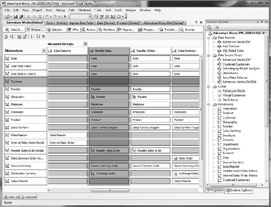
They—the sales and customer dimensions—have no relationship defined. So any use of the Customer dimension against the Reseller Sales measure group won't slice the underlying data, which is the behavior that we saw in Exercise 6-1. At this stage, there most likely doesn't exist any way to identify customers from the reseller data we have. If that turns out to be a critical business need, an analyst will have to go back to the data warehouse group and have that data added to the cubes, if it even exists (the resellers may not report customer data back through the supply chain).
So we see that a complex cube structure can lead to confused and frustrated end users. That is one of the key reasons for preferring a star schema—to easily ensure that every dimension does in fact link to the fact table.
Note
The Enterprise Edition of Analysis Services offers a powerful feature called Perspectives that allows us to address this potential complexity without creating numerous additional cubes. You'll look at this feature in Chapter 7.
Now that you have a basic understanding of where dimensions fit in the grand scheme of things, let's dive down and start looking at working with dimensions in Analysis Services, specifically focusing on building dimensions in BIDS.
You can create a dimension at any time in BIDS just by right-clicking the Dimensions folder and selecting New Dimension, which will open the Dimension Wizard. Alternatively, you can link a dimension, which enables you to create a pointer to a dimension defined in another database. By using linked dimensions, you can maintain "standard" dimension definitions in a database, and then link to them from other cubes as necessary. Finally, dimensions can be implicitly created when you run the cube wizard (you'll look at this in Chapter 7).
Dimensions can either be defined from the data in a data warehouse, or they can be designed in the Analysis Services database solution. In the latter case, the dimension and its attributes are laid out in BIDS, and then the schema generation wizard will create the underlying data tables to support the dimension. (The next step will be to design the ETL to move data from the data sources into the designed schema.) Follow along in Exercise 6-2 and create a dimension that you'll use later in this chapter.
Create a Dimension
Follow the steps in this exercise to create a dimension on promotion. You'll use the dimension for later exercises in this chapter.
Open the SSAS AdventureWorks project you created in Chapter 5.
In BIDS, open the AdventureWorks DW2008 data source view.
Let's add the table we're going to use for our dimension: right-click on the design surface and select Add/Remove Tables. (Alternatively, open the Data Source View menu and select Add/Remove Tables.)
In the Add/Remove Tables Wizard, select the DimPromotion table and click the right-arrow (>) button to move that table to the Included Objects list.
Click the OK button. The DimPromotion table should appear in the data source view, with a relationship to the Reseller Sales table. (If its connector runs behind another table, you can move it to a more convenient location.)
Right-click the DimPromotion table and select Properties. Change the Friendly Name to Promotions.
Save the data source view.
In the Solution Explorer, right-click Dimensions and click New Dimension.
If you see the Welcome to the Dimension Wizard page, click the Next button.
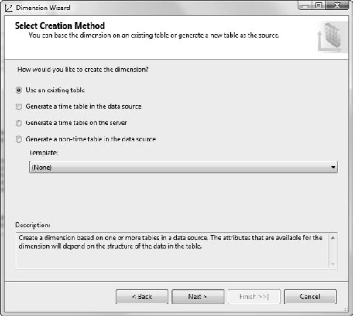
In the Select Creation Method page (Figure 6-13), keep the default of Use an Existing Table and then click the Next button.
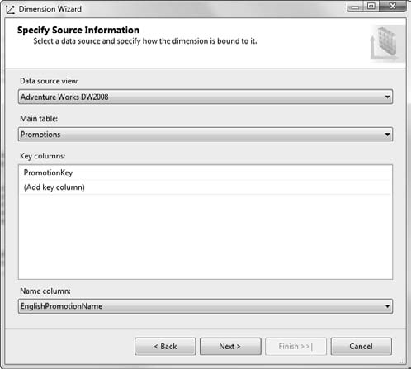
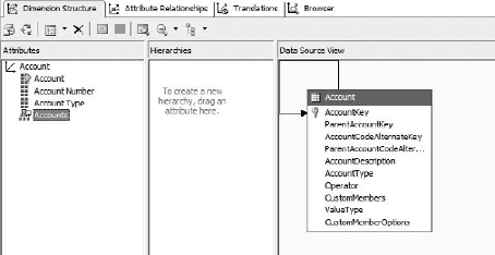
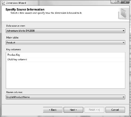
In the Specify Source Information page, the Adventure Works DW2008 data source view should be selected. Select Promotions for the Main table. Leave the default—PromotionKey—as the key column. Change the Name column to EnglishPromotionName (Figure 6-14).
Click the Next button.
In the Select Dimension Attributes page, select attributes in accordance with Table 6-1.
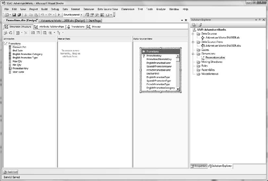
Review the Completing the Wizard page and then click the Finish button. You should end up in the Dimension design surface, which should look like Figure 6-15.
Note that on the left side, the attributes that we indicated weren't browsable are grayed out.
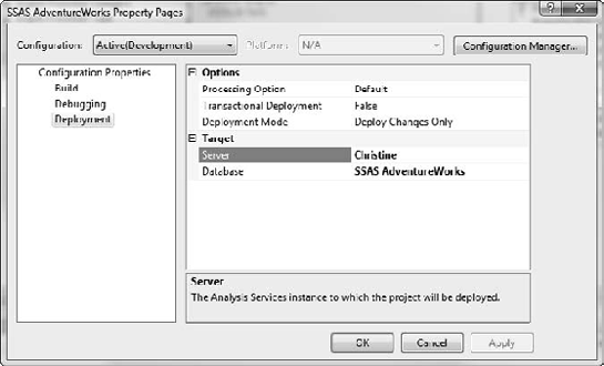
Let's process this dimension. First you'll need to set your deployment server: right-click on SSAS AdventureWorks in the Solution Explorer and select Properties.
In the property pages (Figure 6-16), select Deployment and then enter the name of your server for the Server property (or leave it as localhost if you are working on your SSAS server).
Select the Build menu and then Deploy SSAS AdventureWorks to deploy the solution to the server.
Now either click the Process button (

When the Process Dimension window comes up, click Run. (We'll dive into this window in depth in Chapter 8.)
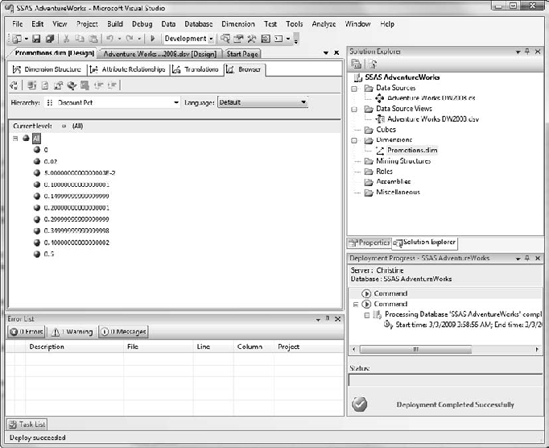
Now we can browse our dimension. In the dimension designer, click the Browser tab.
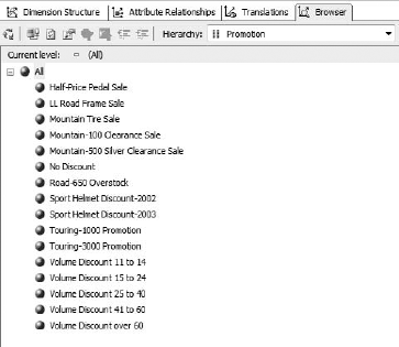
You should see a single member labeled All. Expand it by clicking the [+] icon next to it. You should see something like Figure 6-17.
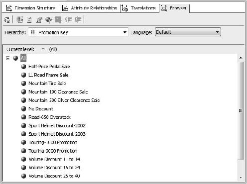
That's odd. Hold on—look at the Hierarchy selection. These are the available Discount Percentages. Change the selection to Promotion Key and open the tree again (Figure 6-18).
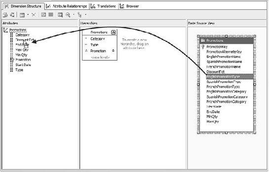
This looks more like a list of dimensions. So how do we make them come up first? We'll use a little trickery. Let's also clean up the dimension a bit. Click the Dimension Structure tab again.
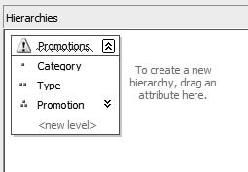
Right-click English Promotion Category, select Rename, and rename it Category.
Similarly, rename English Promotion Type to Type, and Promotion Key to Promotion.
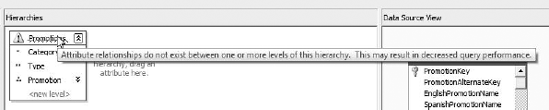
Now we're going to create a hierarchy. Drag Category to the Hierarchies section in the middle of the designer. This will create a Hierarchy container. Drag Type to the <new level> area under Category.
Finally, drag Promotion under Type.
Right-click Hierarchy and select Rename. Rename the hierarchy Promotions. It should look like Figure 6-19.
Note that little blue squiggle under Promotions in the hierarchy. See the upcoming section, "Analysis Management Objects (AMO) Warnings," for more about that. For now don't worry about it.
Save the dimension and process it again.
Click the Browser tab. (You will likely have to click on the Reconnect link in the yellow bar at the bottom to refresh the connection.)
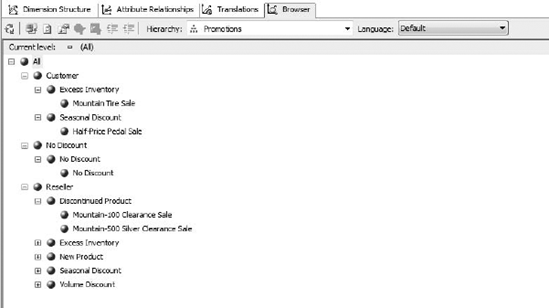
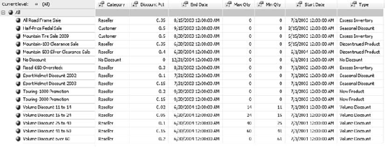
In the Hierarchy tab, select Promotions.
Note that now the promotions are all structured in an easy-to-browse tree (see Figure 6-20).
In this exercise, we talked a lot about attributes and hierarchies. Let's take a deeper look at what they are and how they factor into cube design.
In Exercise 6-2, we see a little blue squiggle in a hierarchy. When we mouse over it, we see a warning (Figure 6-21). This is an Analysis Management Objects (AMO) warning, a new feature in BIDS 2008. AMO warnings are best-practice recommendations to aid in design of Analysis Services cubes. In this case, the warning is pointing out that there is no relationship defined between the Type and Promotion attributes (more on this in the "Attributes" section later in this chapter).
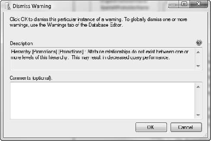
BIDS has dozens of design warning rules that it runs against OLAP designs as you work. The warnings will show up as you work. AMO warnings won't keep you from saving or processing cubes or dimensions. You can choose to ignore warnings, either on a case-by-case basis, or you can dismiss a warning globally.
To dismiss a warning, open the Error List pane (View menu
To view the status of warnings in a database, right-click the database name (the project in the Solution Explorer) and select Edit Database. In the designer that opens, click the Warnings tab (Figure 6-23).
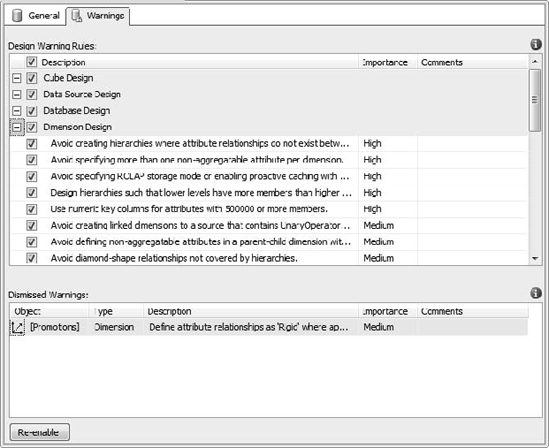
The top section lists the design warning rules available. They're grouped by type of object (Cube, Data Source, and so on), and ranked by importance. You can come in and deselect rules that you don't want enforced. In the lower window are the warnings you've dismissed for the current database (including comments you made when you dismissed them). You can highlight a dismissed warning and click the Re-enable button to put the warning back in place.
Now that you've built a dimension, let's dig into the features and properties. These are accessible by right-clicking on the dimension name in the attributes pane on the left, in Visual Studio, and selecting Properties. The following subsections describe each of the properties that you see.
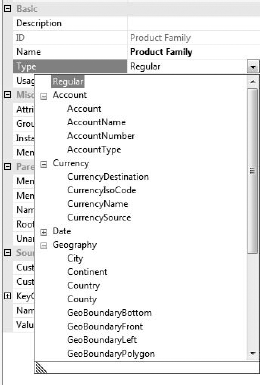
You can flag a dimension with a type—the default is Regular. For the most part, the dimension type is an indicator for client applications on how to treat a dimension. For example, if a dimension is the Customer type, a client application may provide a way to map the dimension to contact cards or a personnel selector-type control. Note that Account, Currency, and Time dimension types do have special handling built into SSAS—we'll look at them separately.
The dimension types are as follows:
- Account:
This dimension represents a chart of accounts (revenues, losses, profits, expenses, and so forth). An Account dimension type can be managed such that specific account types are positive or negative solely based on the account definition.
- Bill of Materials:
A Bill of Materials type will contain manufacturing or inventory information (unit of measure, cost, packaging).
- Channel:
Used in retail sales, a Channel dimension will indicate the sales channel used (wholesale, retail, partners).
- Currency:
The Currency dimension is designed to reflect the financial requirements of dealing with international transactions. SSAS has a currency-conversion feature to manage these transactions.
- Customer:
A Customer dimension will have standard attributes for customers and contact information.
- Geography:
If you want to designate attributes as addresses, cities, and zip codes, then set the dimension type as Geography. You can also have spatial data types in a Geography dimension type.
- Organization:
Employee names, positions, offices, and branches can all be defined in an Organization dimension.
- Product:
A Product dimension will have attribute types for brands, SKUs, and product categories. You can also add attributes for product start and end dates.
- Promotion:
If you need to group facts by the type of deal the buyer got, you can use a Promotion dimension type, including minimum and maximum quantities, start and end dates, percentage discounts, and so on.
- Quantitative:
Quantitative is more a general description than an actual dimension type, and more of a collection of measurement-oriented attributes (volume, weight, color, maximum, minimum, and so forth) than anything else.
- Rates:
Generally a dimension for measuring exchange rates.
- Scenario:
Scenarios are a fascinating capability of an OLAP solution. Because any dimension can "slice" the fact data into exclusive collections (sales in Europe, North America, or Asia), we can create a dimension solely for creating scenarios. For example, a scenario may have members for "5 percent growth," "No growth," and "5 percent decline." Selecting each member then groups the data for that scenario. You'll revisit the concept of scenarios when you look at writeback in Chapter 7.
- Time:
A Time dimension represents a calendar—days, weeks, months, quarters, years. The Time dimension is very special, as we've seen previously, and we'll cover time dimension types specifically later in the chapter.
- Utility:
A Utility dimension is basically a catchall for some aspect of the data that may not be reflected in the business rules.
Each of these dimension types has a host of matching attribute types (Figure 6-24). In general, you can "mix and match" attribute types with dimension types, though some of the special types can be used only in their matching dimension type. If you mismatch types, you'll get an AMO warning on the dimension.
After you've set a dimension type and assigned attribute types, OLAP client applications can leverage known dimension types in business logic. For example, a sales and marketing analysis tool could pull promotion and channel dimensions from your cubes and align them with the analysis system.
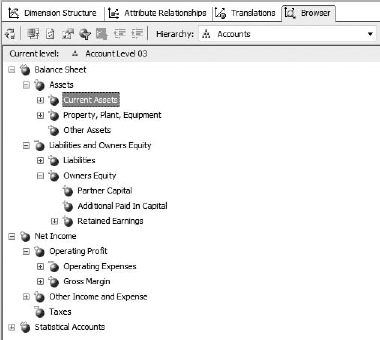
I mentioned that Account, Currency, and Time dimension types are special. In addition to being able to be leveraged by client applications, each of these dimensions can be specified within SSAS to work in special ways. Let's open AdventureWorks and look at the Account dimension (Figure 6-25). Note that the table in the data source view is self-referential. It has a field that is a foreign key for the table's primary key, to indicate the parent account. This creates the recursive hierarchy of accounts in the dimension.
Now let's look at the dimension browser (Figure 6-26). You might not notice at first, but various accounts have plus or minus signs on their icons in the browser. That's because the DBA set up account business intelligence on the dimension. When you run the Add Business Intelligence Wizard (Dimension menu), it walks you through mapping an accounts table to built-in logic for standard accounts. In addition, the UnaryOperatorColumn was set to the Operator column of the Account table. In a parent-child hierarchy dimension, setting the Unary Operator on the parent attribute indicates to Analysis Services to use that column to determine how to aggregate that member.
Currency dimensions have similar logic that can be added via the business intelligence wizard. The wizard is pretty straightforward. You will want a table of exchange rates by time period to handle the automatic currency conversion. One aspect you will have to know is your preferred method of handling local currencies. SSAS will want one of the following three scenarios:
- Many-to-many:
All transactions are recorded in the local currency. Currency conversion is applied at the cube level and can target many currencies.
- Many-to-one:
All transactions are recorded in the local currency. Conversions are applied at the cube level to the corporate standard currency.
- One-to-many:
All transactions are recorded in a single currency. The conversion is applied at the cube level with multiple target currencies.
So if all your sales are reported in the local currency, you can set up a currency dimension and conversion rate table, apply the business intelligence wizard, and you can roll up aggregated sales figures with conversions automatically applied.
This section of properties refers to how Analysis Services should handle errors that crop up while processing the dimension. Think of a dimension as a lookup table—one thing that's necessary is a primary key value to link the dimension and subordinate attributes to records in the cube. So when processing the dimension (reading in the data, parsing it for attributes and relationships, and then caching the dimension data), if multiple records have the same key value, SSAS will throw an error.
You can indicate how to handle the error here. The default action is to ignore the error and continue processing. You can see how this may cause problems, so you might want to change this to either ReportAndContinue or ReportAndStop if you have a data source where you expect you may get duplicates. Both IgnoreError and ReportAndContinue will leverage the KeyErrorAction setting—either converting the key to an Unknown catchall value or discarding the record.
This setting indicates how Analysis Services should handle queries or calculations that reference a member that doesn't exist in the dimension. The default setting is Default, which means the error will be handled in accordance with the settings in Analysis Services and the cube. You can also specifically set this to error out or ignore the error.
These options govern how the dimension is processed. You should generally leave the setting for ProcessingGroup at the default value of ByAttribute. ByTable is used for a small subset of cases generally involving very large dimensions (millions of rows). Setting ProcessingMode to LazyAggregations will make the dimension available for use while it's still being processed, but as a result, processing will take longer.
ProcessingPriority allows you to prioritize the order in which dimensions are processed. You might want certain dimensions (such as Time) available sooner, for example, while other less-used dimensions are processed afterward.
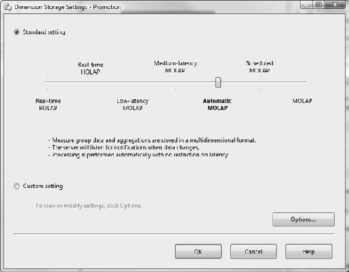
There are two major sections here: StorageMode and ProactiveCaching. Recall the discussion about MOLAP and ROLAP; in Analysis Services you can specify the storage setting for each dimension and measure partition. The two settings here are MOLAP and ROLAP, reflecting the two major options for where dimensions are stored—either in the multidimensional repository or in the relational database.
Where is HOLAP? Well the "hybrid" part of the equation is where the proactive caching comes in. Remember that MOLAP stores the dimension data in the Analysis Services cube, while ROLAP stores the data in the relational store. However, with MOLAP we can also specify proactive caching. With proactive caching, SSAS rebuilds the dimension either when the source data changes, when signaled by a client application, or on scheduled intervals.
If you click the builder button [...] next to the ProactiveCaching setting, you'll open the Dimension Storage Settings dialog box (Figure 6-27). Here you can choose either one of the standard settings or a custom setting. The custom options give you some granular control over the cache, and then allow you to control how SSAS should be notified of changes in the underlying data.
The options for notification are as follows:
- SQL Server:
SSAS simply sets a trace on the necessary tables in SQL Server and tracks for data changes. You can select the Specify Tracking Tables check box and explicitly list the tables SSAS should track for changes (remember, all that will happen is that SSAS will rebuild the dimension if any changes to the data in the indicated tables are detected). If you don't specify the tables, Analysis Services will try to determine from the dimension structure which tables to track.
- Client Initiated:
This is pretty close to regular MOLAP—a client calls for the processing to occur.
- Scheduled Polling:
Specify a polling interval, and SSAS will query the data source for changes; if the data has changed, SSAS will rebuild the dimension. You can also specify incremental updates if you need to process only part of a dimension based on data changes.
Let's take a look at how dimension storage works in Exercise 6-3.
Specify Dimension Storage Modes
Follow the steps in this exercise to work through a detailed example showing how to specify dimension storage.
Open the SSAS AdventureWorks project. Double-click on the Promotions dimension to open that.
First let's check out the dimension as it currently works. Click the Browser tab.
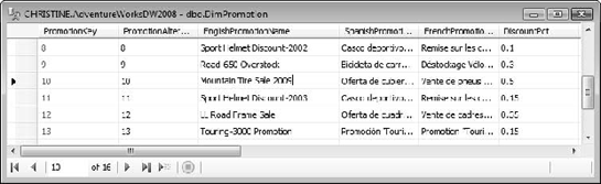
Select the Promotion hierarchy, and then open the tree by clicking the [+] symbol next to the All member (Figure 6-28).
We want to rename the Mountain Tire Sale to Mountain Tire Sale 2009, so let's go change the data in the underlying data table.
Open SQL Server Management Studio.
Connect to the server where the Adventure Works DW2008 database is located (Database Engine connection).
Open the AdventureWorks DW2008 database and then the Tables folder.
Right-click on the dbo.DimPromotion table and select Edit 250 Rows.
Find the promotion where the EnglishPromotionName is Mountain Tire Sale. Change the name to Mountain Tire Sale 2009 (Figure 6-29).
Click the down arrow to leave the row and write the record change to the database.
Now that we've changed the record, let's look at the dimension. Go back to BIDS. (Leave the edit table window open in SSMS—we'll come back to it.)
Refresh the dimension browser (Dimension menu

Process the dimension (Dimension
Let's change the storage. Go back to the Dimension Structure tab.
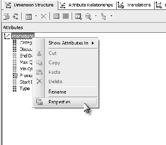
In the left pane (Attributes), right-click on the Promotions at the top of the tree and select Properties (Figure 6-30).
In the Properties pane, under Storage, click the Off option next to ProactiveCaching.
Click the Builder button [...].
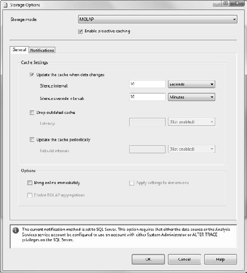
In the Dimension Storage Settings dialog box, select Custom Setting and then click the Options button.
At the top, under the Storage mode drop-down, select the check box for Enable Proactive Caching.
Select the check box labeled Update the Cache When Data Changes. Note the warning at the bottom (Figure 6-31).
Click the Notifications tab. Note that SQL Server is selected and Specify Tracking Tables is not selected. Click the OK button to return to the Dimension Storage Settings dialog box, and click the OK button there. Now we're going to go check our permissions.
What we need is for the account that connects to the SQL Server database to have ALTER TRACE permissions. First let's look at the data source.
In BIDS, double-click on the
Adventure Works DW2008.dsdata source to open the designer.Click the Impersonation Information tab.
The default option is Use the Service Account. This means SSAS will use the service account it's running under to connect to the data source. Click OK to close this dialog.
On the server running Analysis Services, open the Services applet:
Windows Server 2003: Right-click on My Computer, click Manage. In the Computer Management applet, open Services and Applications and click Services.
Windows Server 2008: Right-click on Computer and click Manage. In the Server Manager applet, open Configuration and then click Services.
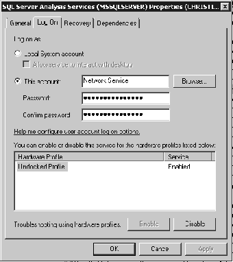
Scroll down to find the SQL Server Analysis Services service. Right-click on it and select Properties.
Click the Log On tab (Figure 6-32).
Note the account named; because the data source is using this account to access the data source, this is the account we have to provide for.
Close the dialog box and management applets.
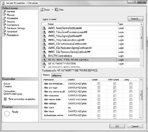
Go back to SQL Server Management Studio.
Right-click on the server in the Object Explorer and select Properties.
In the Properties dialog box, select the Permissions page.
If you scroll down in the Logins or Roles pane, you should see NT AUTHORITYNETWORK SERVICE (Figure 6-33).
Select NT AUTHORITYNETWORK SERVICE and then scroll down in the Permissions pane and select the Alter Trace check box.
Click the OK button.
Return to BIDS and process the dimension (with the new Automatic MOLAP storage setting). Click Yes to "Would you like to build and deploy the project first?"
Click Run when the Process Dimension dialog box shows up. After processing, click Close and then click Close again.
Click the Dimension Structure tab and then the Browser tab. You should get the warning at the bottom of the browser. Click Reconnect.
Let's edit the promotion again—back to SQL Server Management Studio.
Change LL Road Frame Sale to All Road Frame Sale. Remember to click the down arrow to write the change!
Back to BIDS.
In the Dimension menu, click Refresh.
Note that the promotion now indicates All Road Frame Sale and the members are re-sorted!
Our dimension will now automatically update with changes to the database.
The UnknownMember is effectively a catchall where any measures that don't match members in this dimension will be assigned. You have the option as to whether to have an unknown member and whether it's visible. You can also give the member a specific name (for example, Unassigned Sales or Respondents Didn't Answer).
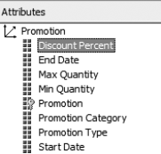
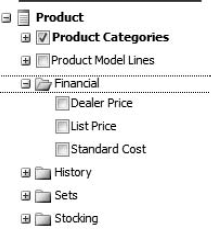
If dimension members are nouns, attributes are adjectives. Let's look back at our Promotion dimension (Figure 6-34). The dimension has attributes for the percentage discount, start and end date, maximum and minimum quantities, promotion category, type, and name. Each of these is amplifying information for each promotion in the dimension.
Attributes are often called containers for dimension members. I find the adjective concept easier to grasp. However, you can see how that approach works—take all the Promotion categories, and each one is something of a "bucket" for the promotions that have that category. However, not every attribute is really a "container"—for example, a Product dimension might have a Price attribute, but grouping by price ($12.95, $13.15, $14.75) wouldn't be that productive.
In addition to enabling drill-down or reporting, attributes are also useful for querying. For example, you can select for all blue bicycles, or use an MDX query like the following, to show sales by product for all products with a list price over $1,000.00. We'll dive into MDX in Chapter 9.
WITH
MEMBER Measures.[List Price] AS [Product].[List Price].CurrentMember.MemberValue

SELECT
{[Date].[Fiscal].[Fiscal Quarter].Members}
ON COLUMNS,

Filter([Product].[Product].Members, (Measures.[List Price]>1000))
ON ROWS

FROM [Adventure Works]
WHERE ([Measures].[Internet Sales Amount])
In the dimension structure, attributes are generally defined by dragging a field from the data source view over to the dimension (Figure 6-35).
For the most part, a dimension consisting of members and attributes is similar to a database table with rows and columns. In fact, you can view the dimension with its attributes as a table: in the browser, selecting Member Properties from the Dimension menu will show all the attributes for the dimension in a table (Figure 6-36).
To really get value out of the collection of attributes in a dimension, we want to build hierarchies and set attribute relationships. Because our users will generally use various attributes in different ways, defining attribute relationships aids the user in seeing relationships in the dimension structure, as well as optimizing performance by defining how attributes are related within the data and by business rule. Let's dig into attribute relationships.
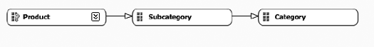
Every attribute in a dimension is related to the key attribute of the dimension, either directly or indirectly (via a relationship with another attribute). By default, when you create a dimension in BIDS, each attribute in the table with the key attribute (in a star schema this would be the only table in the dimension; in a snowflake schema it's the main dimension table) is directly related to the key attribute. The attribute in foreign-key tables bound to the foreign key is also directly related to the key attribute. Finally, attributes based on fields in the foreign-key tables are directly related to the foreign-key attribute (Figure 6-37).
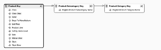
In Figure 6-37, we're looking at the default attribute relationships for a dimension built from the Product, Subcategory, and Category tables. Note that the English Product Subcategory Name and English Product Category Name are each related to the attributes bound to the foreign key in their table, which are related to the Product Key—the key attribute for the dimension.
Attribute relationships should always be built to represent natural hierarchies. A natural hierarchy is simply a one-to-many relationship. Be wary of creating "unnatural hierarchies" with attribute relationships, because these will significantly affect query performance and can even result in inaccurate results.
Note
Also be sure to validate your data; even though a business rule may indicate that data is one-to-many, the actual data may violate the restriction. This is a potential problem with star schemas; with snowflakes, one-to-many relationships can be enforced with database constraints. If you have a star schema and all the attributes for a hierarchy are fields in a table, you could easily end up with many-to-many relationships in the data. So be sure to review your entire BI infrastructure and ensure that checks are in place to validate that the data will do what you think it does.
Building an attribute relationship in the dimension prompts Analysis Services to structure indexes to reflect that relationship. Another thing attribute relationships do is help SSAS understand which indexes not to build. For example, looking back at Figure 6-37, any relationship between category and product can be inferred from the relationships between product and subcategory, then subcategory and category. No explicit relationship needs to be built between product and category.
Attribute relationships can be rigid or flexible. A flexible relationship indicates that the attribute relationship can change over time. When an attribute relationship is flexible, aggregations under that relationship are dropped and recomputed during incremental updates. If the relationship is rigid, the relationships won't be recomputed. Exercise 6-4 presents an example of creating a dimension with attribute relationships.
Warning
If the relationship between attributes with a rigid relationship actually changes, Analysis Services will throw an error during incremental processing.
Create a Dimension with Attribute Relationships
The steps that follow walk you through the process of creating a dimension, and then of creating attribute relationships in that dimension. Let's create the Product dimension for our project.
Right-click on the Dimensions folder in the Solution Explorer and select New Dimension.
In the Dimension Wizard, if you see the Welcome to the Dimension Wizard message, click Next.
On the Select Creation Method page, select Use an Existing Table and click Next.
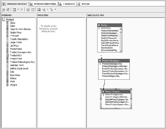
On the Specify Source Information page, select the Adventure Works DW2008 data source view, Product for the main table, and EnglishProductName for the Name column (Figure 6-38).
Click the Next button.
The Related Tables page will detect thatthe Product Subcategory and Product Category tables are linked to the Product table. Leave them selected and click the Next button.
On the Select Dimension Attributes page, select attributes as in Table 6-2.
Table 6.2. Selecting Attributes
Attribute Name
Enable Browsing
Attribute Type
Product Key
Yes
Regular
Color
Yes
Regular
Safety Stock Level
No
Regular
Reorder Point
No
Regular
List Price
Yes
Regular
Size
Yes
Regular
Weight
Yes
Regular
Days To Manufacture
Yes
Regular
Product Line
Yes
Regular
Dealer Price
Yes
Regular
Class
Yes
Regular
Style
Yes
Regular
Model Name
Yes
Regular
Large Photo
No
Regular
English Description
No
Regular
Start Date
No
Slowly Changing Dimension—Date
End Date
No
Slowly Changing Dimension—End Date
Status
No
Slowly Changing Dimension—Status
Product Subcategory Key
Yes
Regular
Product Category Key
Yes
Regular
When you're finished, click the Next button.
Review the construction in the Completing the Wizard page, leave the name Product, and click Finish.
You should end up with a dimension that looks like Figure 6-39.
We want to make the key values more descriptive and appropriate for end users. Click on the Product Key attribute.
Right-click on Product Key in the left-hand attributes pane, and select Rename.
Change the name to Product.
Check the properties for this attribute. The NameColumn property should be Product.EnglishProductName. This way, the user sees proper name values instead of key numbers in the list of Products.
Rename Product Category Key to Category and Product Subcategory Key to Subcategory the same way.
Change the NameColumn property for Category to EnglishProductCategoryName.
Change the NameColumn property for Subcategory to EnglishProductSubcategoryName.
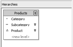
Now let's create a hierarchy: drag the Category attribute to the Hierarchies pane. Then drag the Subcategory attribute to the <new level> area under it, and the Product attribute under that.
Click the hierarchy title bar and change the name to Products (Figure 6-40).
You should see a warning line (blue squiggle) under the Products title in the hierarchy. That's because there's no attribute relationship between the levels of the hierarchy. Click the Attribute Relationships tab.
Drag the Product attribute over the Subcategory attribute and drop it; then drag the Subcategory attribute over the Category attribute. The result should look like Figure 6-41.
Because a Product will always be in a given Subcategory, and a given Subcategory will always be in the same Category, those relationships can be rigid. Right-click on each relationship arrow, select Relationship Type, and then Rigid.
Note that the Attribute Relationships pane shows all relationships, most of which are to the key attribute of Product.
Click the Dimension Structure tab and then click the List Price attribute.
Change the properties for the attribute: DiscretizationBucketCount to 5, DiscretizationMethod to Automatic.
Process the dimension and then check it out in the browser. Note that the List Price hierarchy now consists of five ranges instead of a number of discrete values—that's the result of setting discretization buckets.
Look at the Products hierarchy and make sure you can navigate down categories, subcategories, and products.
Save the project; we'll keep using it.
Let's take a look at the properties for an attribute. Select an attribute and then view the Properties pane (right-click and then select Properties). Let's work down the Properties pane and look at some of the more significant properties. Here's the list:
- AttributeHierarchyDisplayFolder:
This is a free-text value. Any value you type in here will create a folder in the list of attribute hierarchies available (see Figure 6-42).
- AttributeHierarchyEnabled, AttributeHierarchyVisible:
The Enabled property indicates whether the attribute can be used at all for grouping measures. If an attribute is not visible but is enabled, it won't show up in client applications but can be used in MDX expressions.
- DefaultMember:
Indicates which member is selected when the dimension is selected.
- OrderBy, OrderByAttribute:
OrderBy indicates what to use to sort the attribute values (the attribute's key, name, or the key or name of another attribute). If you select AttributeKey or AttributeName, you will also have to enter the name of another attribute to use for sorting.
We'll cover the properties in the "Parent-Child Dimensions" section that follows.
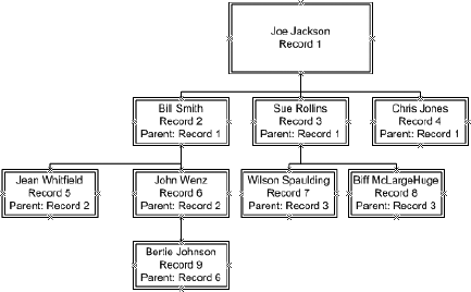
If you have to deal with employees in a company, or records in a file system, you're probably familiar with the concept of recursive data structures. Basically, in these structures, one of the fields annotates parent or owner, and the structure links to itself. Traversing a structure like this gives you a traditional tree or organizational chart type arrangement (see Figure 6-43).
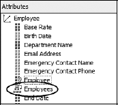
As you can tell, this kind of structure invites interesting challenges. However, Analysis Services handles it very easily. When you create a dimension that has a self-referring relationship, Analysis Services automatically creates a parent-child hierarchy in the dimension. That attribute is marked as a parent attribute type, and has an icon as seen in Figure 6-44.
There are five specific properties relating to parent-child dimensions:
- MembersWithData:
Here you can select whether nonleaf data will be hidden or visible. The leaf members are the members that have no children (at the "bottom" of the hierarchy). Generally in an OLAP measure, all the values are at the leaf level; nonleaf members have values that are the result of aggregating the leaf values. For example, subcategory sales are the result of adding together the sales of all the products in the subcategory; nobody actually sells a subcategory. However, in parent-child dimensions, often nonleaf members will have values of their own. In a sales organization hierarchy, sales managers may also make sales. So how do you show both the rollup of the manager's subordinates and the manager's sales? If you indicate NonLeafDataVisible, SSAS deals with this by creating a "data member" that is a leaf member directly under the manager, containing the data for the manager.
- MembersWithDataCaption:
Here you can give a template for the data member used when you indicate that nonleaf data is visible in a hierarchy. You can type any string—an asterisk will be replaced with the name of the member above. See Figure 6-45.
- NamingTemplate:
If you look back to Figure 6-43, note that there are four levels in the hierarchy. In a normal SSAS hierarchy, you would annotate each level by the attribute name (Categories, Subcategories, Products). However, in a parent-child hierarchy, there are no natural names—every level is Employees. So Analysis Services creates a dynamic name based on this template. You can enter multiple terms separated by semicolons. When you process the dimension, Analysis Services will assign the terms starting at the first level. When SSAS runs out of terms, it will keep using the last term but appending index numbers: 1, 2, 3, and so on.
- RootMemberIf:
If you think about the way this hierarchy is built, one thing to wonder is how to find where it starts. That's what this setting is about. You can establish the root member by setting its parent ID to itself, leaving the value blank, or leaving it undefined. With this setting, you can choose which method to use, or if all three are acceptable.
- UnaryOperatorColumn:
Remember our Account dimension? Each level had an indicator as to whether it should be added or subtracted to the aggregation. This property is where you indicate which column to use that holds those operators (see Figure 6-46).
If you choose to use parent-child dimensions, be sure that your intended client applications handle them gracefully. You definitely want to keep them in the first round of requirements and test to verify that everything works as you expect. Now let's move on to our final special case for dimensions, and perhaps the most important—the Time dimension.
The Time dimension is a special case in OLAP technology. If you think about a calendar as a dimension, there are several facts about it that differentiate it from other dimensions:
There are specific directions for forward (newer) and back (older).
The members create a continuous range (1–31 January, 1–28 February, and so forth).
When semiadditive measures calculate different dimensions in different ways, the Time dimension is usually the one dimension that is different from the others (inventory levels are added in other dimensions, and averaged in the Time dimension).
Rolling averages over time have meaning (rolling averages by product do not).
The concept of to date exists, which allows analysis of time periods not yet ended (year to date, quarter to date).
As a result, OLAP engines are designed to recognize Time dimensions and work with them. And SQL Server Analysis Services is no different. A basic Time dimension will be based on a table with date data—a date field, which will be a normal DateTime value, then a number of additional fields to enable Analysis Services to create hierarchies as well as perform various kinds of date math. The data source view table will then contain additional calculated fields to build out the full definition of a date model (see Figure 6-47).
Date dimensions can have multiple calendars. In addition to the standard calendar, you can also have the following:
- Fiscal calendar:
Many companies have financial reporting years that end on dates other than January 1. The fiscal calendar reflects the position in the fiscal year. For example, the US federal government has a fiscal year that starts on October 1. So October/November/December of 2008 is the first fiscal quarter of fiscal year 2009 (Q1FY09).
- Reporting calendar:
A reporting calendar follows a standard quarterly structure in which two months in the quarter have four weeks, and the other month has five. You can indicate which month has five weeks by selecting the month pattern (445, 454, or 544).
- Manufacturing calendar:
This calendar has thirteen "months" of four weeks each, divided into four quarters (three quarters with three months, one with four). You can set when the calendar starts as well as which quarter has the extra "month."
- ISO 8601 calendar:
This calendar follows the ISO standard calendar, which establishes a fixed number of seven-day weeks within a year, and establishes the start date of the year, based on the Gregorian calendar.
Being able to use and combine these calendars can provide a powerful new analytic capability to the end users, who may need to relate financial data to manufacturing data, or calendar data to reporting data.
You have several methods of creating time tables in BIDS:
- Generate a time table in the data source:
Using the new Dimension Wizard, this will create a Time dimension mapped to a data source view. If you generate the schema, it will also generate the table in the data source, optionally fill it with date data, and map it in the data source view.
- Generate a time table on the server:
This will generate the time table on the SSAS server, in the event you don't have permissions to create a table on the data source server.
- Roll your own:
Perhaps you already have a table populated with every date, or need to build your own for some other reason. It's possible, but painful.
The resulting structure of a Date dimension is shown in Figure 6-48.
The easiest way to understand dimensions is to create one, so let's embark on our last exercise. Exercise 6-5 shows how to create Date dimensions for use in analyzing time-based data.
Create a Date Dimension
Follow the steps in this exercise to create a Date dimension. Such dimensions are useful in analyzing historical data that has been recorded over time.
Open the SSAS AdventureWorks project.
Right-click on the Dimensions folder and select New Dimension.
If you get the Welcome to the Dimension Wizard pane, click the Next button.
Select the option Generate a Time Table in the Data Source. Then click Next.
The calendar day options indicate how much of the dimension data source will be prepopulated with dates. The data in AdventureWorks goes from mid-2001 to mid-2004, so let's set the start date as 1/1/2001 and the end date as 12/31/2005.
Note
As time goes on, you will need a process and mechanism in place to generate additional date data for the underlying table.
Leave the first day of the week as Sunday. In the time periods, select Year, Quarter, Month, Week, and Date. The screen should look like Figure 6-49.
Click the Next button.
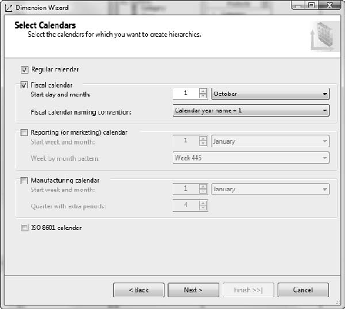
On the Select Calendars page, select the Regular Calendar and Fiscal Calendar check boxes. For the Fiscal Calendar, set the Start Day and Month to 1 October (see Figure 6-50).
Click the Next button.
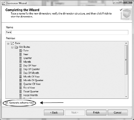
Change the name to Date. Select the check box labeled Generate Schema Now near the bottom (Figure 6-51). This runs the wizard to create the data tables and data source view.
Click the Finish button.
The Schema Generation Wizard opens; if you're on the Welcome page, click the Next button.
On the Specify Target page, select Use Existing Data Source View and ensure that Adventure Works DW2008 is selected.
Click the Next button.
On the Subject Area Database Schema Options page, leave the defaults and click the Next button.
The Specify Naming Conventions page enables you to define naming conventions for the table that will be created in the database. Leave the defaults and click the Next button.
On the final page, click the Finish button.
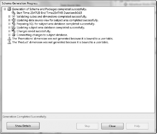
Figure 6-52 shows the status page after a successful run. Note the warnings for the Promotion and Product dimensions. The wizard tries to generate a schema for every dimension in the database. Because those two dimensions are already bound to tables, they weren't touched.
Click the Close button.
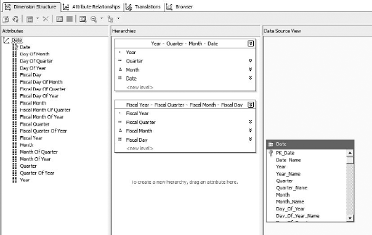
Now you should see a Date dimension in your solution (Figure 6-53). We'll connect it up in the next chapter.
Save the solution.

So that's our tour of dimensions in SQL Server 2008 Analysis Services. Remember that defining your dimensional space is the key to developing a solid OLAP solution. Dimensions are like the tent poles, and in Chapter 7, we'll look at the fabric of the tent—that is to say, measures.