![]()
The amount of data stored in relational databases is growing exponentially every year. Customers are collecting more data, and processing and retaining it for a longer amount of time. We, as database professionals, are working with databases that have become larger over time.
From a development standpoint, database size is not that critical. Non-optimized queries time out regardless of the database size. However, from a database administration standpoint, management of the large databases introduces additional challenges. Data partitioning helps to address some of these challenges.
In this chapter, we will discuss the reasons we want to partition data, and we will cover the different techniques of data partitioning what are available in SQL Server. We will focus on the practical implementation scenarios and typical data partitioning use-cases in SQL Server.
Reasons to Partition Data
Let’s assume that our system stores data in a large non-partitioned table. This approach dramatically simplifies development. All data is in the same place, and you can read the data from and write the data to the same table. With such a design, however, all of the data is stored in the same location. The table resides in a single filegroup, which consists of one or multiple files stored on the same disk array. Even though, technically speaking, you could spread indexes across different filegroups or data files across different disk arrays; it introduces additional database management challenges, reduces the recoverability of data in case of a disaster, and rarely helps with performance.
At the same time, in almost every system, data, which is stored in large tables, can be separated into two different categories: operational and historical. The first category consists of the data for the current operational period of the company and handles most of the customers’ requests in the table. Historical data, on the other hand, belongs to the older operational periods, which the system must retain for various reasons, such as regulations and business requirements, among others.
Most activity in the table is performed against operational data, even though it can be very small compared to the total table size. Obviously, it would be beneficial to store operational data on the fast and expensive disk array. Historical data, on the other hand, does not need such I/O performance.
When data is not partitioned, you cannot separate it between disk arrays. You either have to pay extra for the fast storage you do not need, or compromise and buy larger but slower storage. Unfortunately, the latter option occurs more often in the real world.
It is also common for operational and historical data to have different workloads. Operational data usually supports OLTP, the customer-facing part of the system. Historical data is mainly used for analysis and reporting. These two workloads produce different sets of queries, which would benefit from a different set of indexes.
Unfortunately, it is almost impossible to index a subset of the data in a table. Even though you can use filtered indexes and/or indexed views, both approaches have several limitations. In most cases, you have to create a set of indexes covering both workloads in the table scope. This requires additional storage space and introduces update overhead for operational activity in the system. Moreover, volatile operational data requires different and more frequent index maintenance as compared to static historical data, which is impossible to implement in such a case.
Data compression is another important factor to consider. Static historical data would usually benefit from page-level data compression, which can significantly reduce the storage space required. Moreover, it could improve the performance of queries against historical data in non CPU-bound systems by reducing the number of I/O operations required to read the data. At the same time, page-level data compression introduces unnecessary CPU overhead when the data is volatile.
![]() Tip In some cases, it is beneficial to use page compression even with volatile operational data when it saves signigicant amount of space and the system works under a heavy I/O load. As usual, you should test and monitor how it affects the system.
Tip In some cases, it is beneficial to use page compression even with volatile operational data when it saves signigicant amount of space and the system works under a heavy I/O load. As usual, you should test and monitor how it affects the system.
Unfortunately, it is impossible to compress part of the data in a table. You would either have to compress the entire table, which would introduce CPU overhead on operational data, or keep the historical data uncompressed at additional storage and I/O cost.
In cases of read-only historical data, it could be beneficial to exclude it from FULL database backups. This would reduce the size of the backup file and I/O and network load during backup operations. Regrettably, partial database backups work on the filegroup level, which makes it impossible when the data is not partitioned.
The Enterprise Edition of SQL Server supports piecemeal restore, which allows you to restore the database and bring it online on a filegroup-by-filegroup basis. It is great to have a disaster recovery strategy that allows you to restore operational data and make it available to customers separately from the historical data. This could significantly reduce the disaster recovery time for large databases.
Unfortunately, such a design requires separation of operational and historical data between different filegroups, which is impossible when the data is not partitioned.
![]() Note We will discuss backup and disaster recovery strategies in greater detail in Chapter 30, “Designing a Backup Strategy.”
Note We will discuss backup and disaster recovery strategies in greater detail in Chapter 30, “Designing a Backup Strategy.”
Another important factor is statistics. As you will remember, the statistics histogram stores a maximum of 200 steps, regardless of the table size. As a result, the histogram steps on large tables must cover a bigger interval of key values. It makes the statistics and cardinality estimation less accurate, and it can lead to suboptimal execution plans in the case of large tables. Moreover, SQL Server tracks the number of changes in the statistics columns and by default requires this to exceed about 20 percent of total number of rows in the table before the statistics become outdated. Therefore, statistics are rarely updated automatically in large tables.
![]() Note You can use undocumented trace flag T2371 in SQL Server 2008R2 SP1 and above to make the statistics update threshold dynamic.
Note You can use undocumented trace flag T2371 in SQL Server 2008R2 SP1 and above to make the statistics update threshold dynamic.
That list is by no means complete, and there are other factors as to why data partitioning is beneficial, although either of the aforementioned reasons is enough to start considering it.
When to Partition?
Database professionals often assume that data partitioning is required only for very large databases (VLDB). Even though database size definitely matters, it is hardly the only factor to consider.
Service-level agreements (SLA)are one of the key elements in the decision to partition or not. When a system has an availability-based SLA clause, data partitioning becomes essential. The duration of possible downtime depends on how quickly you can recover a database and restore it from a backup after disaster. That time depends on the total size of the essential filegroups that need to be online for the system to be functional. Data partitioning is the only approach that allows you to separate data between different filegroups and use a piecemeal restore to minimize downtime.
A performance-based SLA clause is another important factor. Data partitioning can help address some of the challenges of performance tuning. For example, by partitioning data between multiple tables, you will improve the accuracy of statistics and you can use different indexing strategies for historical and operational data. Moreover, data partitioning allows you to implement a tiered storage approach and put the operational part of the data on faster disks, which improves the performance of the system. We will discuss tiered storage in greater detail later in the chapter.
The key point to remember is that you should not rely on database size as the only criteria for partitioning. Consider data partitioning merely to be a tool that helps you address some of the challenges. This tool can be useful regardless of database size.
Nevertheless, data partitioning comes at a cost. It changes the execution plans of queries and often requires code refactoring. You need to keep this in mind, especially in the case of new development. When you expect a system to collect a large amount of data in the future, it is often better to implement data partitioning at a very early development stage. Even though data partitioning introduces development overhead, such overhead may be much smaller than that which is involved in code refactoring and the retesting of the production system with large amounts of data.
![]() Note The cost of data partitioning is especially important for independent software vendors (ISV) who are deploying a system to a large number of customers. It is a mistake to assume that data partitioning can be implemented transparently to the client applications. Even though table partitioning does not require any code changes, it affects execution plans and can lead to performance issues, which requires code refactoring and, therefore, a separate code base to support.
Note The cost of data partitioning is especially important for independent software vendors (ISV) who are deploying a system to a large number of customers. It is a mistake to assume that data partitioning can be implemented transparently to the client applications. Even though table partitioning does not require any code changes, it affects execution plans and can lead to performance issues, which requires code refactoring and, therefore, a separate code base to support.
Finally, it is often very hard if not impossible to partition the data while keeping the database online and available to users. Moving large amounts of data around can be time consuming and can lead to long downtimes. This is another argument for implementing data partitioning during the initial stage of development.
Data Partitioning Techniques
There are two data partitioning techniques available in SQL Server: partitioned tables and partitioned views. Let’s look at them in detail.
![]() Note In this chapter, we will use an Order Entry system, which stores order information for two and a half years, as our example. Let’s assume that we want to partition the data on a monthly basis and that our operational period consists of two months: May and June 2014.
Note In this chapter, we will use an Order Entry system, which stores order information for two and a half years, as our example. Let’s assume that we want to partition the data on a monthly basis and that our operational period consists of two months: May and June 2014.
Partitioned Tables
Table partitioning is an Enterprise Edition feature, which was introduced in SQL Server 2005. You can think of partitioned tables as logical tables, which consist of multiple individual internal physical tables-partitions. That terminology—logical and physical table—is not standard, although it describes it perfectly.
![]() Note Technically speaking, every table in SQL Server is partitioned. When a table is not partitioned by the user, SQL Server treats it as a single-partition table internally.
Note Technically speaking, every table in SQL Server is partitioned. When a table is not partitioned by the user, SQL Server treats it as a single-partition table internally.
SQL Server tracks allocation units, such as IN-ROW, ROW-OVERFLOW, and LOB data, separately for each partition. For example, a table with 10 partitions would have 30 different IAM chains per data file—one per allocation unit per partition.
There are two additional database objects that are used together with table partitioning. A Partition Function specifies boundary values, which are the criteria on how data needs to be partitioned. A Partition Scheme specifies filegroups in which physical partition tables are stored.
Listing 15-1 shows the code that creates partitioned table OrdersPT with the data partitioned on a monthly basis. This code assumes that the database has four different filegroups: FG2012 and FG2013 store data for years 2012 and 2013, respectively. FG2014 stores data for the first four months of 2014. Finally, the FASTSTORAGE filegroup stores operational data starting from May 2014.
Listing 15-1. Creating a partitioned table
create partition function pfOrders(datetime2(0))
as range right for values
('2012-02-01', '2012-03-01','2012-04-01','2012-05-01','2012-06-01'
,'2012-07-01','2012-08-01','2012-09-01','2012-10-01','2012-11-01'
,'2012-12-01','2013-01-01','2013-02-01','2013-03-01','2013-04-01'
,'2013-05-01','2013-06-01','2013-07-01','2013-08-01','2013-09-01'
,'2013-10-01','2013-11-01','2013-12-01','2014-01-01','2014-02-01'
,'2014-03-01','2014-04-01','2014-05-01','2014-06-01','2014-07-01'),

create partition scheme psOrders
as partition pfOrders
to (
FG2012 /* FileGroup to store data <'2012-02-01' */
,FG2012 /* FileGroup to store data >='2012-02-01' and <'2012-03-01' */
,FG2012,FG2012,FG2012,FG2012,FG2012
,FG2012,FG2012,FG2012,FG2012,FG2012
,FG2013 /* FileGroup to store data >='2013-01-01' and <'2013-02-01' */
,FG2013,FG2013,FG2013,FG2013,FG2013
,FG2013,FG2013,FG2013,FG2013,FG2013,FG2013
,FG2014 /* FileGroup to store data >='2014-01-01' and <'2014-02-01' */
,FG2014,FG2014,FG2014
,FASTSTORAGE /* FileGroup to store data >='2014-05-01' and <'2014-06-01' */
,FASTSTORAGE /* FileGroup to store data >='2014-06-01' and <'2014-07-01' */
,FASTSTORAGE /* FileGroup to store data >='2014-07-01' */
);

create table dbo.OrdersPT
(
        OrderId int not null,
        OrderDate datetime2(0) not null,
        OrderNum varchar(32) not null,
        OrderTotal money not null,
        CustomerId int not null,
        /* Other Columns */
);

create unique clustered index IDX_OrdersPT_OrderDate_OrderId
on dbo.OrdersPT(OrderDate, OrderId)
with
(
        data_compression = page on partitions(1 to 28),
        data_compression = row on partitions(29 to 31)
)
on psOrders(OrderDate);

create nonclustered index IDX_OrdersPT_CustomerId
on dbo.OrdersPT(CustomerId)
with
(
        data_compression = page on partitions(1 to 28),
        data_compression = row on partitions(29 to 31)
)
on psOrders(OrderDate);
You control how boundary values are stored by specifying either the RANGE LEFT or RANGE RIGHT parameter of the partition function. In our example, we are using the RANGE RIGHT parameter, which indicates that the boundary value is stored on the right partition. With this option, if 2012-02-01 is the first boundary value, the leftmost partition stores the data, which is prior to that date. All values, which are equal to the boundary value, are stored in the second from the left partition. Alternatively, if we used the RANGE LEFT parameter, the boundary value data would be stored in the left partition.
Figure 15-1 shows the physical data layout of the OrdersPT table.

Figure 15-1. Data layout of dbo.OrdersPT table
Each partition can reside on its own filegroup and have its own data compression method. However, all partitions have exactly the same schema and set of indexes controlled by the logical table. Moreover, SQL Server does not maintain individual statistics at the partition level. There is a single 200-step histogram on the index, regardless of whether it is partitioned or not.
![]() Note SQL Server 2014 can track the number of statistics column updates at the partition level and marks statistics as outdates when it exceeds the update threshold on an individual partition. This behavior needs to be enabled with the statistics_incremental index and incremental statistics options respectively.
Note SQL Server 2014 can track the number of statistics column updates at the partition level and marks statistics as outdates when it exceeds the update threshold on an individual partition. This behavior needs to be enabled with the statistics_incremental index and incremental statistics options respectively.
Table partitioning can be implemented in a transparent manner to the client applications. The code continues to reference the logical table while SQL Server manages the internal data layout under the hood.
![]() Note There are still some cases when you need to reference individual partitions during the query optimization stage. We will talk about these cases later in the chapter.
Note There are still some cases when you need to reference individual partitions during the query optimization stage. We will talk about these cases later in the chapter.
You can create new (split) or drop existing (merge) partitions by altering the partition scheme and functions. The code in Listing 15-2 merges the two leftmost and split rightmost partitions in the OrdersPT table. After the split, the two rightmost partitions of the table will store data with an OrderDate for July 2014, equal to or greater than 2014-08-01, respectively.
Listing 15-2. Splitting and merging partitions
/* Merging two left-most partitions */
alter partition function pfOrders() merge range('2012-02-01')
go

/* Splitting right-most partition */
-- Step 1: Altering partition scheme - specifying FileGroup
-- where new partition needs to be stored
alter partition scheme psOrders next used [FASTSTORAGE];

-- Step 2: Splitting partition function
alter partition function pfOrders() split range('2014-08-01'),
One of the most powerful features of table partitioning is the ability to switch partitions between tables. That dramatically simplifies the implementation of some operations, such as purging old data or importing data into the table.
![]() Note We will discuss implementing data purge and sliding window patterns later in the chapter.
Note We will discuss implementing data purge and sliding window patterns later in the chapter.
Listing 15-3 shows you how to import new data into the table MainData by switching another staging table, StagingData, as the new partition. This approach is very useful when you need to import data from external sources into the table. Even though you can insert data directly into the table, a partition switch is a metadata operation, which allows you to minimize locking during the import process.
Listing 15-3. Switching a staging table as the new partition
create partition function pfMainData(datetime)
as range right for values
('2014-02-01', '2014-03-01','2014-04-01','2014-05-01','2014-06-01'
,'2014-07-01','2014-08-01','2014-09-01','2014-10-01','2014-11-01'
,'2014-12-01'),

create partition scheme psMainData
as partition pfMainData
all to (FG2014);

/* Even though we have 12 partitions - one per month, let's assume
that only January-April data is populated. E.g. we are in the middle
of the year */
create table dbo.MainData
(
        ADate datetime not null,
        ID bigint not null,
        CustomerId int not null,
        /* Other Columns */
        constraint PK_MainData
        primary key clustered(ADate, ID)
        on psMainData(ADate)
);

create nonclustered index IDX_MainData_CustomerId
on dbo.MainData(CustomerId)
on psMainData(ADate);

create table dbo.StagingData
(
        ADate datetime not null,
        ID bigint not null,
        CustomerId int not null,
        /* Other Columns */
        constraint PK_StagingData
        primary key clustered(ADate, ID),

        constraint CHK_StagingData
        check(ADate >= '2014-05-01' and ADate < '2014-06-01')
) on [FG2014];

create nonclustered index IDX_StagingData_CustomerId
on dbo.StagingData(CustomerId)
on [FG2014];

/* Switching partition */
alter table dbo.StagingData
switch to dbo.MainData
partition 5;
![]() Note We will discuss locking in greater detail in Part 3, “Locking, Blocking, and Concurrency.”
Note We will discuss locking in greater detail in Part 3, “Locking, Blocking, and Concurrency.”
Both tables must have exactly the same schema and indexes. The staging table should be placed in the same filegroup with the destination partition in the partitioned table. Finally, the staging table must have a CHECK constraint, which prevents values outside of the partition boundaries.
As you probably noticed, all nonclustered indexes have been partitioned in the same way as clustered indexes. Such indexes are called aligned indexes. Even though there is no requirement to keep indexes aligned, SQL Server would not be able to switch partitions when a table has non-aligned, nonclustered indexes defined.
Finally, the partition switch operation does not work if a table is referenced by foreign key constraints defined in other tables. Nevertheless, a partition switch is allowed when the table itself has foreign key constraints referencing other tables.
Partitioned Views
Unlike partitioned tables, partitioned views work in every edition of SQL Server. In such schema, you create individual tables and combine data from all of them via a partitioned view using the union all operator.
![]() Note SQL Server allows you to define partitioned views combining data from multiple databases or even SQL Server instances. The latter case is called Distributed Partitioned Views. The coverage of such scenarios is outside of the scope of the book. However, they behave similarly to partitioned views defined in a single database scope.
Note SQL Server allows you to define partitioned views combining data from multiple databases or even SQL Server instances. The latter case is called Distributed Partitioned Views. The coverage of such scenarios is outside of the scope of the book. However, they behave similarly to partitioned views defined in a single database scope.
Listing 15-4 shows an example of data partitioning of the Orders entity using a partitioned view approach.
Listing 15-4. Creating partitioned views
create table dbo.Orders2012_01
(
        OrderId int not null,
        OrderDate datetime2(0) not null,
        OrderNum varchar(32) not null,
        OrderTotal money not null,
        CustomerId int not null,
        /* Other Columns */
        constraint PK_Orders2012_01
        primary key clustered(OrderId),

        constraint CHK_Orders2012_01
        check (OrderDate >= '2012-01-01' and OrderDate < '2012-02-01')
) on [FG2012];

create nonclustered index IDX_Orders2012_01_CustomerId
on dbo.Orders2012_01(CustomerId)
on [FG2012];

create table dbo.Orders2012_02
(
        OrderId int not null,
        OrderDate datetime2(0) not null,
        OrderNum varchar(32) not null,
        OrderTotal money not null,
        CustomerId int not null,
        /* Other Columns */
        constraint PK_Orders2012_02
        primary key clustered(OrderId)
        with (data_compression=page),

        constraint CHK_Orders2012_02
        check (OrderDate >= '2012-02-01' and OrderDate < '2012-03-01')
) on [FG2012];

create nonclustered index IDX_Orders2012_02_CustomerId
on dbo.Orders2012_02(CustomerId)
with (data_compression=page)
on [FG2012];

/* Other tables */

create table dbo.Orders2014_06
(
        OrderId int not null,
        OrderDate datetime2(0) not null,
        OrderNum varchar(32) not null,
        OrderTotal money not null,
        CustomerId int not null,
        /* Other Columns */
        constraint PK_Orders2014_06
        primary key clustered(OrderId)
        with (data_compression=row),

        constraint CHK_Orders2014_06
        check (OrderDate >= '2014-06-01' and OrderDate < '2014-07-01')
) on [FASTSTORAGE];

create nonclustered index IDX_Orders2014_04_CustomerId
on dbo.Orders2014_06(CustomerId)
with (data_compression=row)
on [FASTSTORAGE]
go

create view dbo.Orders(OrderId, OrderDate, OrderNum
        ,OrderTotal, CustomerId /*Other Columns*/)
with schemabinding
as
        select OrderId, OrderDate, OrderNum
                ,OrderTotal, CustomerId /*Other Columns*/
        from dbo.Orders2012_01

        union all

        select OrderId, OrderDate, OrderNum
                ,OrderTotal, CustomerId /*Other Columns*/
        from dbo.Orders2012_02

        /* union all -- Other tables */
        union all

        select OrderId, OrderDate, OrderNum
                ,OrderTotal, CustomerId /*Other Columns*/
        from dbo.Orders2014_06;
Figure 15-2 shows the physical data layout of the tables.

Figure 15-2. Data layout with a partitioned view approach
As you can see, different tables can be placed into different filegroups, which can even be marked as read-only if needed. Each table can have its own set of indexes and maintain individual, more accurate statistics. Moreover, each table can have its own schema. This is beneficial if operational activities require tables to have additional columns, for data processing, for example, which you can drop afterwards. The difference in schemas can be abstracted on the partitioned view level.
It is extremely important to have CHECK constraints defined in each table. Those constraints help SQL Server avoid accessing unnecessary tables while querying the data. Listing 15-5 shows an example of queries against a partitioned view.
Listing 15-5. Queries against partitioned view
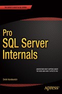
select count(*) from dbo.Orders;
select count(*) from dbo.Orders where OrderDate = '2014-06-03'
As you can see in Figure 15-3, the first query requires SQL Server to access all of the tables from the partitioned view. Alternatively, the second query has OrderDate as a parameter, which allows SQL Server to pinpoint the single table that needs to be queried.
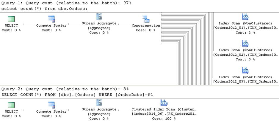
Figure 15-3. Execution plans of the queries against a partitioned view
You should always add predicates, which reduce the number of tables to be processed by the queries. Let’s look at a practical example and, as the first step, create another entity called OrderLineItems. Obviously, you would like to partition it in the same way as the Orders entity; that is, on a monthly basis.
![]() Tip You should partition related entities and place them in filegroups in a way that supports piecemeal restore and which allows you to bring entities online together.
Tip You should partition related entities and place them in filegroups in a way that supports piecemeal restore and which allows you to bring entities online together.
Listing 15-6 shows the code that creates the set of tables and the partitioned view. Even though the OrderDate column is redundant in the OrderLineItems table, you need to add it to all of the tables in order to create a consistent partitioning layout with the Orders tables.
Listing 15-6. OrderLineItems partition view
create table dbo.OrderLineItems2012_01
(
        OrderId int not null,
        OrderLineItemId int not null,
        OrderDate datetime2(0) not null,
        ArticleId int not null,
        Quantity decimal(9,3) not null,
        Price money not null,
        /* Other Columns */

        constraint CHK_OrderLineItems2012_01
        check (OrderDate >= '2012-01-01' and OrderDate < '2012-02-01'),

        constraint FK_OrderLineItems_Orders_2012_01
        foreign key(OrderId)
        references dbo.Orders2012_01(OrderId),

        constraint FK_OrderLineItems2012_01_Articles
        foreign key(ArticleId)
        references dbo.Articles(ArticleId)
);

create unique clustered index IDX_Orders2012_01_OrderId_OrderLineItemId
on dbo.OrderLineItems2012_01(OrderId, OrderLineItemId)
on [FG2012];

create nonclustered index IDX_Orders2012_01_ArticleId
on dbo.OrderLineItems2012_01(ArticleId)
on [FG2012];

/* Other tables */

create view dbo.OrderLineItems(OrderId, OrderLineItemId
        ,OrderDate, ArticleId, Quantity, Price)
with schemabinding
as
        select OrderId, OrderLineItemId, OrderDate
                ,ArticleId, Quantity, Price
        from dbo.OrderLineItems2012_01

        /*union all other tables*/

        union all

        select OrderId, OrderLineItemId, OrderDate
                ,ArticleId, Quantity, Price
        from dbo.OrderLineItems2014_06;
Let’s assume that you have a query that returns a list of orders that includes a particular item bought by a specific customer in January 2014. The typical implementation of the query is shown in Listing 15-7.
Listing 15-7. Selecting a list of customer orders with a specific item: Non-optimized version
select o.OrderId, o.OrderNum, o.OrderDate, i.Quantity, i.Price
from dbo.Orders o join dbo.OrderLineItems i on
        o.OrderId = i.OrderId
where
        o.OrderDate >= '2014-01-01' and
        o.OrderDate < '2014-02-01' and
        o.CustomerId = @CustomerId and
        i.ArticleId = @ArticleId
As you can see in Figure 15-4, SQL Server has to perform an index seek in every OrderLineItems table while searching for line item records. Query Optimizer is not aware that all required rows are stored in the OrderLineItems2014_01 table.

Figure 15-4. Execution plans of a non-optimized query
You can optimize this query by adding another join predicate on the OrderDate column, as shown in Listing 15-8. CHECK constraints allow Query Optimizer to eliminate access to the tables, which cannot store the data for a particular month. The execution plan is shown in Figure 15-5.
Listing 15-8. Selecting a list of customer orders with a specific item: Optimized version
select o.OrderId, o.OrderNum, o.OrderDate, i.Quantity, i.Price
from dbo.Orders o join dbo.OrderLineItems i on
        o.OrderId = i.OrderId and
        o.OrderDate = i.OrderDate
where
        o.OrderDate >= '2014-01-01' and
        o.OrderDate < '2014-02-01' and
        o.CustomerId = @CustomerId and
        i.ArticleId = @ArticleId
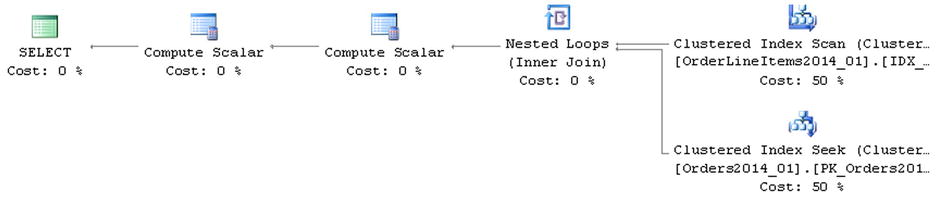
Figure 15-5. Execution plans of an optimized query
Unfortunately, in most cases, using partitioned views requires modifications of the client code, especially when you update the data. In some cases, you can update the data directly through the view; however, partitioned views have a few restrictions in order to be updateable. For example, tables from the view should have a CHECK constraint that defines the partitioning criteria and a column from that constraint must be part of the primary key.
Another important requirement is that view should deliver all columns from the tables and that is it; no calculated columns are allowed. With such a requirement, you are unable to have tables with different schemas abstracting the difference on the view level.
Even when all requirements are met, and an updateable view can be created, there is still a supportability issue. You should be extremely careful when altering the view to avoid the situation where alteration accidentally breaks the client code.
Another way to make the view updateable is by defining an INSTEAD OF trigger on the view. However, such an approach will often perform less efficiently than updating the base tables directly from the client code. Moreover, with the client code, you can update different tables simultaneously from the different threads, which could improve the performance of batch operations.
Comparing Partitioned Tables and Partitioned Views
Table 15-1 compares partitioned tables and partitioned views in further detail.
Table 15-1. Comparison of partitioned tables and partitioned views
Partitioned Tables |
Partitioned Views |
|---|---|
Enterprise and Developer editions only |
All editions |
Maximum 1,000 or 15,000 partitions depending on SQL Server version |
Maximum 255 tables/partitions |
Same table schema and indexes across all partitions |
Every table/partition can have its own schema and set of indexes |
Statistics kept at the table level |
Separate statistics per table/partition |
No partition-level online index rebuild prior to SQL Server 2014 |
Online index rebuild of the table/partition with Enterprise edition of SQL Server |
Transparent to client code (some query refactoring may be required) |
Usually requires changes in the client code |
Transparent for replication |
Requires changes in publications when a new table/partition is created and/or an existing table/partition is dropped |
As you can see, partitioned views are more flexible compared to partitioned tables. Partitioned views work in every edition of SQL Server, which is important for Independent Software Vendors who are deploying systems to multiple customers with different editions of SQL Server. However, partitioned views are harder to implement, and they often require significant code refactoring in existing systems.
System supportability is another factor. Consider the situation where you need to change the schema of the entity. With partitioned tables, the main logical table controls the schema and only one ALTER TABLE statement is required. Partitioned views, on the other hand, require multiple ALTER TABLE statements—one per underlying table.
It is not necessarily a bad thing, though. With multiple ALTER TABLE statements, you acquire schema modifications (SCH-M) locks at the individual table level, which can reduce the time the lock is held and access to the table is blocked.
![]() Note We will discuss schema locks in greater detail in Chapter 23, “Schema Locks.”
Note We will discuss schema locks in greater detail in Chapter 23, “Schema Locks.”
Sometimes you can abstract schema changes at the partition view level, which allows you to avoid altering some tables. Think about adding a NOT NULL column with a default constraint as an example. In SQL Server 2005-2008R2, this operation would modify every data row in the table and keep the schema modification (SCH-M) lock held for the duration of the operation. It also generates a large amount of transaction log activity.
In the case of partitioned views, you can alter operational data tables only by using a constant with historical data tables in the view. Listing 15-9 illustrates such an approach. Keep in mind that such an approach prevents a partitioned view from being updateable.
Listing 15-9. Abstracting schema changes in the partitioned view
alter table dbo.Orders2014_06
add IsReviewed bit not null
        constraint DEF_Orders2014_06_IsReviewed
        default 0;

alter view dbo.Orders(OrderId, OrderDate, OrderNum
        ,OrderTotal, CustomerId, IsReviewed)
with schemabinding
as
        select OrderId, OrderDate, OrderNum
                ,OrderTotal, CustomerId, 0 as [IsReviewed]
        from dbo.Orders2012_01

        /* union all -- Other tables */

        union all

        select OrderId, OrderDate, OrderNum
                ,OrderTotal, CustomerId, IsReviewed
        from dbo.Orders2014_06
Using Partitioned Tables and Views Together
You can improve the supportability of a system and reduce the number of required tables by using partitioned tables and partitioned views together. With such an approach, you are storing historical data in one or more partitioned tables and operational data in regular table(s), combining all of them into partitioned view.
Listing 15-10 shows such an example. There are three partitioned tables: Orders2012, Orders2013, and Orders2014, which store historical data partitioned on a monthly basis. There are also two regular tables storing operational data: Orders2014_05 and Orders2014_06.
Listing 15-10. Using partitioned tables and views together
create partition function pfOrders2012(datetime2(0))
as range right for values
('2012-02-01', '2012-03-01','2012-04-01','2012-05-01','2012-06-01'
,'2012-07-01','2012-08-01','2012-09-01','2012-10-01','2012-11-01'
,'2012-12-01'),

create partition scheme psOrders2012
as partition pfOrders2012
all to ([FG2012]);

create table dbo.Orders2012
(
        OrderId int not null,
        OrderDate datetime2(0) not null,
        OrderNum varchar(32) not null,
        OrderTotal money not null,
        CustomerId int not null,
        /* Other Columns */
        constraint CHK_Orders2012
        check(OrderDate >= '2012-01-01' and OrderDate < '2013-01-01')
);

create unique clustered index IDX_Orders2012_OrderDate_OrderId
on dbo.Orders2012(OrderDate, OrderId)
with (data_compression = page)
on psOrders2012(OrderDate);

create nonclustered index IDX_Orders2012_CustomerId
on dbo.Orders2012(CustomerId)
with (data_compression = page)
on psOrders2012(OrderDate);
go

/* dbo.Orders2013 table definition */

create partition function pfOrders2014(datetime2(0))
as range right for values
('2014-02-01', '2014-03-01','2014-04-01','2014-05-01','2014-06-01'
,'2014-07-01','2014-08-01','2014-09-01','2014-10-01','2014-11-01'
,'2014-12-01'),

create partition scheme psOrders2014
as partition pfOrders2014
all to ([FG2014]);

create table dbo.Orders2014
(
        OrderId int not null,
        OrderDate datetime2(0) not null,
        OrderNum varchar(32) not null,
        OrderTotal money not null,
        CustomerId int not null,
        /* Other Columns */
        constraint CHK_Orders2014
        check(OrderDate >= '2014-01-01' and OrderDate < '2014-05-01')
);

create unique clustered index IDX_Orders2014_OrderDate_OrderId
on dbo.Orders2014(OrderDate, OrderId)
with (data_compression = page)
on psOrders2014(OrderDate);

create nonclustered index IDX_Orders2014_CustomerId
on dbo.Orders2014(CustomerId)
with (data_compression = page)
on psOrders2014(OrderDate);

create table dbo.Orders2014_05
(
        OrderId int not null,
        OrderDate datetime2(0) not null,
        OrderNum varchar(32) not null,
        OrderTotal money not null,
        CustomerId int not null,
        /* Other Columns */
        constraint CHK_Orders2014_05
        check(OrderDate >= '2014-05-01' and OrderDate < '2014-06-01')
);

create unique clustered index IDX_Orders2014_05_OrderDate_OrderId
on dbo.Orders2014_05(OrderDate, OrderId)
with (data_compression = row)
on [FASTSTORAGE];

create nonclustered index IDX_Orders2014_05_CustomerId
on dbo.Orders2014_05(CustomerId)
with (data_compression = row)
on [FASTSTORAGE]

/* dbo.Orders2014_06 table definition */

create view dbo.Orders(OrderId, OrderDate, OrderNum
        ,OrderTotal, CustomerId /*Other Columns*/)
with schemabinding
as
        select OrderId, OrderDate, OrderNum
                ,OrderTotal, CustomerId /*Other Columns*/
        from dbo.Orders2012

        union all

        select OrderId, OrderDate, OrderNum
                ,OrderTotal, CustomerId /*Other Columns*/
        from dbo.Orders2013

        union all

        select OrderId, OrderDate, OrderNum
                ,OrderTotal, CustomerId /*Other Columns*/
        from dbo.Orders2014

        union all

        select OrderId, OrderDate, OrderNum
                ,OrderTotal, CustomerId /*Other Columns*/
        from dbo.Orders2014_05

        union all

        select OrderId, OrderDate, OrderNum
                ,OrderTotal, CustomerId /*Other Columns*/
        from dbo.Orders2014_06;
It is worth mentioning that table Orders2014 is partitioned on a monthly basis up to end of the year, even though it stores the data up to the operational period, which starts in May. CHECK constraints in that table indicate this.
The data layout is shown in Figure 15-6.
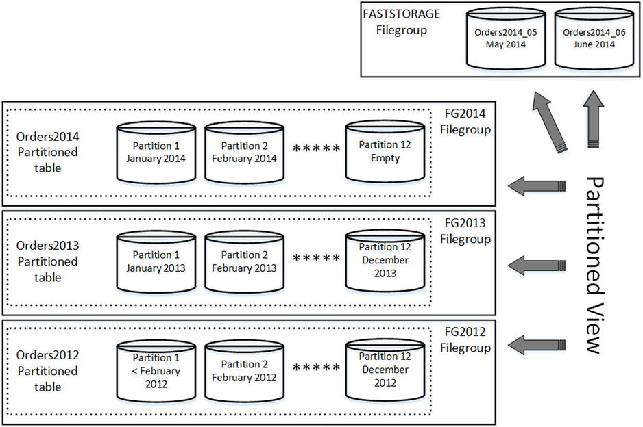
Figure 15-6. Using partitioned tables and views together: Data layout
As you can see, such an approach dramatically reduces the number of tables as compared to a partitioned views implementation, keeping the flexibility of partitioned views intact.
One of the key benefits of data partitioning is reducing storage costs in the system. You can achieve this in two different ways. First, you can reduce the size of the data by using data compression on the historical part of the data. Moreover, and more importantly, you can separate data between different storage arrays in the system.
It is very common to have different performance and availability requirements for different data in the system. In our example, it is possible to have 99.99 percent availability and 20ms latency SLAs defined for operational data. However, for the older historical data, the requirements could be quite different. For example, orders from 2012 must be retained in the system without any performance requirements, and the availability SLA is much lower than it is for operational data.
You can design a data layout and storage subsystem based on these requirements. Figure 15-7 illustrates one possible solution. You can use a fast SSD-based RAID-10 array for the FASTSTORAGE filegroup, which contains operational data. Data for January-April 2014 is relatively static, and it could be stored on the slower RAID-5 array using 15,000-RPM disks. Finally, you can use slow and cheap 5,400-RPM disks in the RAID-1 array for the data from the years 2013 and 2012.
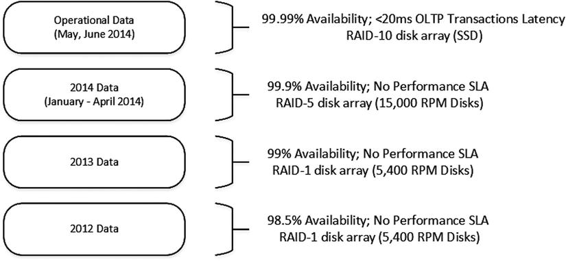
Figure 15-7. Tiered storage
Tiered storage can significantly reduce the storage costs of the system. Finally, yet importantly, it is also much easier to get an approved budget allocation to buy a lower-capacity fast disk array due to its lower cost.
The key question with tiered storage design is how to move data between different tiers when the operational period changes, keeping the system online and available to customers. Let's look at the available options in greater detail.
Moving Non-Partitioned Tables Between Filegroups
You can move a non-partitioned table to another filegroup by rebuilding all of the indexes using the new filegroup as the destination. This operation can be done online in the Enterprise Edition of SQL Server with the CREATE INDEX WITH (ONLINE=ON, DROP_EXISTING=ON) command. Other sessions can access the table during the online index rebuild. Therefore the system is available to customers.
![]() Note Online index rebuild acquires schema modification (SCH-M) lock during the final phase of execution. Even though this lock is held for a very short time, it can increase locking and blocking in very active OLTP systems. SQL Server 2014 introduces the concept of low-priority locks, which can be used to improve system concurrency during online index rebuild operations. We will discuss low-priority locks in detail in Chapter 23, “Schema Locks.”
Note Online index rebuild acquires schema modification (SCH-M) lock during the final phase of execution. Even though this lock is held for a very short time, it can increase locking and blocking in very active OLTP systems. SQL Server 2014 introduces the concept of low-priority locks, which can be used to improve system concurrency during online index rebuild operations. We will discuss low-priority locks in detail in Chapter 23, “Schema Locks.”
Unfortunately, there are two caveats associated with online index rebuild. First, even with the Enterprise Edition, SQL Server 2005-2008R2 does not support online index rebuild if an index has large-object (LOB) columns defined, such as (n)text, image, (n)varchar(max), varbinary(max), xml, and others.
The second issue is more complicated. Index rebuild does not move LOB_DATA allocation units to the new filegroup. Let’s look at an example and create a table that has an LOB column on the FG1 filegroup. Listing 15-11 shows the code for this.
Listing 15-11. Moving a table with an LOB column to a different filegroup: Table creation
create table dbo.RegularTable
(
        OrderDate date not null,
        OrderId int not null identity(1,1),
        OrderNum varchar(32) not null,
        LobColumn varchar(max) null,
        Placeholder char(50) null,
) textimage_on [FG1];

create unique clustered index IDX_RegularTable_OrderDate_OrderId
on dbo.RegularTable(OrderDate, OrderId)
on [FG1];
As a next step, let’s check that all allocation units are residing in the FG1 filegroup. The code for this is shown in Listing 15-12. You can see the result of the query in Figure 15-8.
Listing 15-12. Moving a table with an LOB column to a different filegroup: Checking allocation units placement
select
        p.partition_number as [Partition]
        ,object_name(p.object_id) as [Table]
        ,filegroup_name(a.data_space_id) as [FileGroup]
        ,a.type_desc as [Allocation Unit]
from
        sys.partitions p join sys.allocation_units a on
                p.partition_id = a.container_id
where
        p.object_id = object_id('dbo.RegularTable')
order by
        p.partition_number
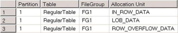
Figure 15-8. Allocation units placement after table creation
Now let’s rebuild the clustered index, moving the data to the FG2 filegroup. The code for doing this is shown in Listing 15-13.
Listing 15-13. Rebuilding the index by moving data to a different filegroup
create unique clustered index IDX_RegularTable_OrderDate_OrderId
on dbo.RegularTable(OrderDate, OrderId)
with (drop_existing=on, online=on)
on [FG2]
Now if you run the query from Listing 15-12 again, you will see the results shown in Figure 15-9. As you can see, the index rebuild moved IN_ROW_DATA and ROW_OVERFLOW_DATA allocation units to the new filegroup, keeping LOB_DATA intact.

Figure 15-9. Allocation units placement after index rebuild
Fortunately, there is a workaround available. You can move LOB_DATA allocation units to another filegroup by performing an online index rebuild using a partition scheme rather than a filegroup as the destination.
Listing 15-14 shows such an approach. As a first step, you need to create a partition function with one boundary value and two partitions in a way that leaves one partition empty. After that, you need to create a partition scheme using a destination filegroup for both partitions and perform an index rebuild into this partition scheme. Finally, you need to merge both partitions by altering the partition function. This is quick metadata operation because one of the partitions is empty.
Listing 15-14. Rebuilding an index in a partition scheme
create partition function pfRegularTable(date)
as range right for values ('2100-01-01'),

create partition scheme psRegularTable
as partition pfRegularTable
all to ([FG2]);

create unique clustered index IDX_RegularTable_OrderDate_OrderId
on dbo.RegularTable(OrderDate, OrderId)
with (drop_existing=on, online=on)
on psRegularTable(OrderDate);

alter partition function pfRegularTable()
merge range('2100-01-01'),
Figure 15-10 shows the allocation units placement after the index rebuild.

Figure 15-10. Allocation units placement after rebuilding the index in the partition scheme
Obviously, this method requires the Enterprise Edition of SQL Server. It also would require SQL Server 2012 or above to work as an online operation because of the LOB columns involved.
Without the Enterprise Edition of SQL Server, your only option for moving LOB_DATA allocation units is to create a new table in the destination filegroup and copy the data to it from the original table.
Moving Partitions Between Filegroups
You can move a single partition from a partitioned table to another filegroup by altering the partition scheme and function. Altering the partition scheme marks the filegroup in which the newly created partition must be placed. Splitting and merging the partition function triggers the data movement.
The way that data is moved between partitions during RANGE SPLIT and RANGE MERGE operations depends on the RANGE LEFT and RANGE RIGHT parameters of the partition function. Let’s look at an example and assume that you have a database with four filegroups: FG1, FG2, FG3, and FG4. You have a partition function in the database that uses RANGE LEFT values, as shown in Listing 15-15.
Listing 15-15. RANGE LEFT partition function
create partition function pfLeft(int)
as range left for values (10,20);

create partition scheme psLeft
as partition pfLeft
to ([FG1],[FG2],[FG3]);

alter partition scheme psLeft
next used [FG4];
In a RANGE LEFT partition function, the boundary values represent the highest value in a partition. When you split a RANGE LEFT partition, the new partition with the highest new boundary value is moved to the NEXT USED filegroup.
Table 15-2 shows a partition and filegroup layout for the various SPLIT operations.
Table 15-2. RANGE LEFT partition function and SPLIT operations
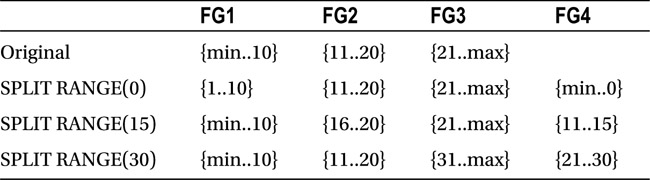
Now let’s look at what happens when you have RANGE RIGHT partition function with the same boundary values, as defined in Listing 15-16.
Listing 15-16. RANGE RIGHT partition function
create partition function pfRight(int)
as range right for values (10,20);

create partition scheme psRight
as partition pfRight
to ([FG1],[FG2],[FG3])
go

alter partition scheme psRight
next used [FG4];
In a RANGE RIGHT partition function, the boundary values represent the lowest value in a partition. When you split a RANGE RIGHT partition, the new partition with the new lowest boundary value is moved to the NEXT USED filegroup.
Table 15-3 shows a partition and filegroup layout for the various SPLIT operations.
Table 15-3. RANGE RIGHT partition function and SPLIT operations
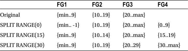
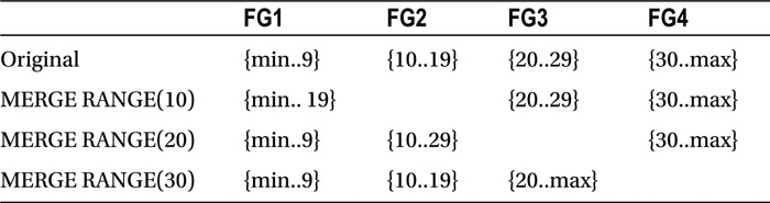
Now let’s look at a MERGE operation and assume that you have partition functions with the boundary values of (10, 20, 30). For a RANGE RIGHT partition function, the data from the right partition is moved to the left partition filegroup. Table 15-4 illustrates this point.
Table 15-4. RANGE LEFT partition function and MERGE operations
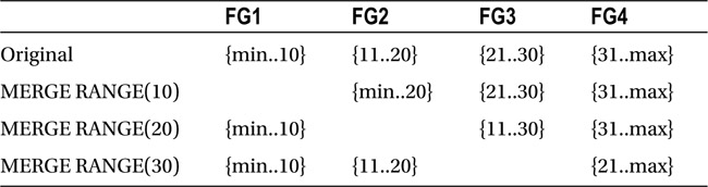
Conversely, with a RANGE LEFT partition function, the data from the left partition is moved to the right partition filegroup, as shown in Table 15-5.
Table 15-5. RANGE RIGHT partition function and MERGE operations
When you move a partition to a different filegroup, you should choose a boundary value to SPLIT and MERGE the partition function based on that behavior. For example, if you want to move a partition that stores May 2014 data in the OrdersPT table from the FASTSTORAGE to the FG2014 filegroup, you need to MERGE and SPLIT a boundary value of 2014-05-01. The partition function is defined as RANGE RIGHT and, as a result, the MERGE operation moves May 2014 data to the partition containing the April 2014 data, which resides on the FG2014 filegroup. Afterward, the SPLIT operation would move the May 2014 data to the filegroup you specified as NEXT USED by altering partition scheme.
You can see the code to accomplish this in Listing 15-17. As a reminder, the OrdersPT table was created in Listing 15-1.
Listing 15-17. Moving data for a single partition
-- Moving May 2014 partition data to April 2014 filegroup
alter partition function pfOrders()
merge range ('2014-05-01'),

-- Marking that next used filegroup
alter partition scheme psOrders
next used [FG2014];

-- Creating new partition for May 2014 moving it to FG2014
alter partition function pfOrders()
split range ('2014-05-01'),
Even though the code is very simple, there are a couple problems with such an approach. First, the data is moved twice when you MERGE and SPLIT a partition function. Another problem is that SQL Server acquires and holds schema modification (SCH-M) lock for the duration of the data movement, which prevents other sessions from accessing the table.
There is no easy workaround for the problem of keeping the table online during data movement. One of the options, shown in Listing 15-18, is to rebuild the indexes using a different partition scheme. Even though this operation can be performed online, it introduces a huge I/O and transaction log overhead because you are rebuilding indexes in the entire table rather than moving a single partition. Moreover, this operation will not work online in SQL Server 2005-2008R2 if the table has LOB columns.
Listing 15-18. Moving data for a single partition
create partition scheme psOrders2
as partition pfOrders
to (
FG2012,FG2012,FG2012,FG2012,FG2012,FG2012,FG2012,FG2012
,FG2012,FG2012,FG2012,FG2012,FG2013,FG2013,FG2013,FG2013
,FG2013,FG2013,FG2013,FG2013,FG2013,FG2013,FG2013,FG2013
,FG2014,FG2014,FG2014,FG2014,FASTSTORAGE,FASTSTORAGE
);

create unique clustered index IDX_OrdersPT_OrderDate_OrderId
on dbo.OrdersPT(OrderDate, OrderId)
with
(
        data_compression = page on partitions(1 to 28),
        data_compression = none on partitions(29 to 31),
        drop_existing = on, online = on
)
on psOrders2(OrderDate);

create nonclustered index IDX_OrdersPT_CustomerId
on dbo.OrdersPT(CustomerId)
with
(
        data_compression = page on partitions(1 to 28),
        data_compression = none on partitions(29 to 31),
        drop_existing = on, online = on
)
on psOrders2(OrderDate);
Another workaround would be to switch the partition to a staging table, moving that table to a new filegroup with an online index rebuild and switching the table back as the partition to the original table. This method requires some planning and additional code to make it transparent to the client applications.
Let’s look more closely at this approach. One of the key elements here is the view that works as another layer of abstraction for the client code, hiding the staging table during the data movement process.
Let’s create a table that stores data for the year 2014, partitioned on a monthly basis. The table stores the data up to April in the FG1 filegroup using FG2 afterwards. You can see the code for doing this in Listing 15-19.
Listing 15-19. Using a temporary table to move partition data: Table and view creation
create partition function pfOrders(datetime2(0))
as range right for values
('2014-02-01','2014-03-01','2014-04-01'
,'2014-05-01','2014-06-01','2014-07-01'),

create partition scheme psOrders
as partition pfOrders
to (FG1,FG1,FG1,FG1,FG2,FG2,FG2);

create table dbo.tblOrders
(
        OrderId int not null,
        OrderDate datetime2(0) not null,
        OrderNum varchar(32) not null,
        OrderTotal money not null,
        CustomerId int not null,
        /* Other Columns */
);

create unique clustered index IDX_tblOrders_OrderDate_OrderId
on dbo.tblOrders(OrderDate, OrderId)
on psOrders(OrderDate);

create nonclustered index IDX_tblOrders_CustomerId
on dbo.tblOrders(CustomerId)
on psOrders(OrderDate);
go

create view dbo.Orders(OrderId, OrderDate, OrderNum
        ,OrderTotal, CustomerId /*Other Columns*/)
with schemabinding
as
        select OrderId, OrderDate, OrderNum
                ,OrderTotal, CustomerId /*Other Columns*/
        from dbo.tblOrders;
As you can see, the script creates an updateable Orders view in addition to the table. All access to the data should be done through that view.
Let’s assume that you want to move May 2014 data to the FG1 filegroup. As a first step, you need to create a staging table and switch May’s partition to there. The table must reside in the FG2 filegroup and have a CHECK constraint defined. The code for accomplishing this is shown in Listing 15-20.
Listing 15-20. Using a temporary table to move partition data: Switching the partition to the staging table
create table dbo.tblOrdersStage
(
        OrderId int not null,
        OrderDate datetime2(0) not null,
        OrderNum varchar(32) not null,
        OrderTotal money not null,
        CustomerId int not null,
        /* Other Columns */
        constraint CHK_tblOrdersStage
        check(OrderDate >= '2014-05-01' and OrderDate < '2014-06-01')
);

create unique clustered index IDX_tblOrdersStage_OrderDate_OrderId
on dbo.tblOrdersStage(OrderDate, OrderId)
on [FG2];

create nonclustered index IDX_tblOrdersStage_CustomerId
on dbo.tblOrdersStage(CustomerId)
on [FG2];

alter table dbo.tblOrders
switch partition 5 to dbo.tblOrdersStage;
Now you have data in two different tables, and you need to alter the view, making it partitioned. That change allows the client applications to read the data transparently from both tables. However, it would prevent the view from being updateable. The simplest way to address this is to create INSTEAD OF triggers on the view.
You can see the code for doing this in Listing 15-21. It shows only one INSTEAD OF INSERT trigger statement in order to save space in this book.
Listing 15-21. Using a temporary table to move partition data: Altering the view
alter view dbo.Orders(OrderId, OrderDate, OrderNum
        ,OrderTotal, CustomerId /*Other Columns*/)
with schemabinding
as
        select OrderId, OrderDate, OrderNum
                ,OrderTotal, CustomerId /*Other Columns*/
        from dbo.tblOrders
        union all
        select OrderId, OrderDate, OrderNum
                ,OrderTotal, CustomerId /*Other Columns*/
        from dbo.tblOrdersStage
go

create trigger dbo.trgOrdersView_Ins
on dbo.Orders
instead of insert
as
        if @@rowcount = 0 return
        set nocount on
        if not exists(select * from inserted)
                return
        insert into dbo.tblOrders(OrderId, OrderDate
                ,OrderNum, OrderTotal, CustomerId)
                select OrderId, OrderDate, OrderNum
                        ,OrderTotal, CustomerId
                from inserted
                where
                        OrderDate < '2014-05-01' or
                        OrderDate >= '2014-06-01'

        insert into dbo.tblOrdersStage(OrderId, OrderDate
                ,OrderNum, OrderTotal, CustomerId)
                select OrderId, OrderDate, OrderNum
                        ,OrderTotal, CustomerId
                from inserted
                where
                        OrderDate >= '2014-05-01' and
                        OrderDate < '2014-06-01'
Now you can move the staging table to the FG1 filegroup by performing an index rebuild, as shown in Listing 15-22. It is worth repeating that if the table has LOB columns, it cannot work as an online operation in SQL Server 2005-2008R2. Moreover, you will need to use a workaround and rebuild the indexes in the new partition scheme to move the LOB_DATA allocation units, as was shown earlier in Listing 15-14.
Listing 15-22. Using a temporary table to move partition data: Moving the staging table
create unique clustered index IDX_tblOrdersStage_OrderDate_OrderId
on dbo.tblOrdersStage(OrderDate, OrderId)
with (drop_existing=on, online=on)
on [FG1];

create nonclustered index IDX_tblOrdersStage_CustomerId
on dbo.tblOrdersStage(CustomerId)
with (drop_existing=on, online=on)
on [FG1];
As the final step, you need to move the tblOrders table May data partition to the FG1 filegroup by merging and splitting the partition function. The partition is empty and a schema modification (SCH-M) lock will not be held for a long time. After that, you can switch the staging table back as a partition to the tblOrders table, drop the trigger, and alter the view again. The code for doing this is shown in Listing 15-23.
Listing 15-23. Using a temporary table to move partition data: Moving the staging table
alter partition function pfOrders()
merge range ('2014-05-01'),

alter partition scheme psOrders
next used [FG1];

alter partition function pfOrders()
split range ('2014-05-01'),

alter table dbo.tblOrdersStage
switch to dbo.tblOrders partition 5;

drop trigger dbo.trgOrdersView_Ins;

alter view dbo.Orders(OrderId, OrderDate, OrderNum
        ,OrderTotal, CustomerId /*Other Columns*/)
with schemabinding
as
        select OrderId, OrderDate, OrderNum
                ,OrderTotal, CustomerId /*Other Columns*/
        from dbo.tblOrders;
The same technique would work if you need to archive data into another table. You can switch the staging table as a partition there as long as the table schemas and indexes are the same.
Moving Data Files Between Disk Arrays
As you can see, there are plenty of limitations that can prevent online cross-filegroup data movement, even in the Enterprise Edition of SQL Server. It is simply impossible to do this in the non-Enterprise editions, which do not support online index rebuild at all.
Fortunately, there is still a workaround that allows you to build tiered storage, regardless of those limitations. You can keep the objects in the same filegroups by moving the filegroup database files to different disk arrays.
There are two ways to implement this. You can manually copy the data files and alter the database to specify their new location. Unfortunately, that approach requires system downtime for the duration of the file copy operation, which can take a long time with large amounts of data.
If downtime is not acceptable, you can move the data online by adding new files to the filegroup and shrinking the original files with the DBCC SHRINK(EMPTYFILE) command. SQL Server moves the data between files transparently to the client applications, keeping the system online, no matter the edition of SQL Server.
Listing 15-24 shows the code for moving data files from filegroup FG2013 to disk S:. It assumes that the filegroup has two files with the logical names Orders2013_01 and Orders2013_02 before the execution.
Listing 15-24. Moving data files between disk arrays
use master
go

alter database OrderEntryDB
add file
(
        name = N'Orders2013_03',
        filename = N'S:Orders2013_03.ndf'
)
to filegroup [FG1];

alter database OrderEntryDB
add file
(
        name = N'Orders2013_04',
        filename = N'S:Orders2013_04.ndf'
)
to filegroup [FG1]
go

use OrderEntryDb
go

-- Step 1: Shrinking and removing first old file
dbcc shrinkfile(Orders2013_01, emptyfile);
alter database OrderEntryDb remove file Orders2013_01
go

-- Step 2: Shrinking and removing second old file
dbcc shrinkfile(Orders2013_02, emptyfile);
alter database OrderEntryDb remove file Orders2013_02
![]() Important Make sure to create new files with the same initial size and auto growth parameters, with growth size specified in MB. This helps SQL Server evenly distribute data across data files.
Important Make sure to create new files with the same initial size and auto growth parameters, with growth size specified in MB. This helps SQL Server evenly distribute data across data files.
There are two caveats with such an approach. When you empty a file with the DBCC SHRINKFILE command, it distributes the data across all other files in the filegroup including files that you will empty and remove in the next steps, which adds unnecessary overhead to the system.
I will try to illustrate it with a set of diagrams. Figure 15-11 shows the original data placement. I am using different shading to distinguish between data from the different files.

Figure 15-11. Data placement after new files have been created
When you run the DBCC SHRINKFILE(Orders2013_01,emptyfile) command, data from the Orders2013_01 file would be moved to three other files, as is shown in Figure 15-12. Part of the data is moved to the Orders2013_02 file even though you are going to remove this file in the next step. This unnecessary data movement from Order2013_01 to Orders2013_02 introduces I/O and transaction log overhead in the system.

Figure 15-12. Data placement after the DBCC SHRINKFILE(Orders2013_01,EMPTYFILE) command and Orders2013_01 file removal
When you run the DBCC SHRINKFILE(Orders2013_02,emptyfile) command, data from the Orders2013_02 file would be moved to remaining data files, as is shown in Figure 15-13.
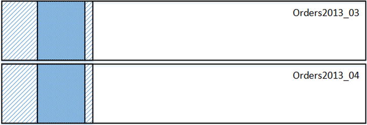
Figure 15-13. Data placement after running the DBCC SHRINKFILE(Orders2013_02,EMPTYFILE) command and Orders2013_02 file removal
Another issue with this approach is index fragmentation. The data in the new data files would be heavily fragmented after the DBCC SHRINKFILE operation. You should perform index maintenance after the data has been moved.
![]() Tip Index REORGANIZE could be a better choice than REBUILD in this case. REORGANIZE is online operation, which would not block access to the table. Moreover, it will not increase size of the data files.
Tip Index REORGANIZE could be a better choice than REBUILD in this case. REORGANIZE is online operation, which would not block access to the table. Moreover, it will not increase size of the data files.
You can monitor the progress of the SHRINK operation by using the script shown in Listing 15-25. This script shows you the currently allocated file size and amount of free space for each of the database files.
Listing 15-25. Monitoring the size of the database files
select
        name as [FileName]
        ,physical_name as [Path]
        ,size / 128.0 as [CurrentSizeMB]
        ,size / 128.0 - convert(int,fileproperty(name,'SpaceUsed')) /
                128.0 as [FreeSpaceMb]
from sys.database_files
Tiered Storage in Action
Table 15-6 shows the available online data movement options for different database objects based on the versions and editions of SQL Server in use.
Table 15-6. Online data movement of database objects based on the SQL Server version and edition
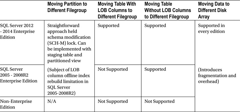
As you can see, it is generally easier to implement online data movement using non-partitioned rather than partitioned tables. This makes the approach that we discussed in the “Using Partitioned Tables and Views Together” section of this chapter as one of the most optimal solutions. With such an approach, you are using non-partitioned tables to store operational data, keeping the historical data in partitioned tables, as was shown in Figure 15-6.
Let’s look at the process of changing the operational period in more depth, assuming that you need to archive May 2014 data and extend the operational period to July 2014.
In the first step shown in Figure 15-14, you move the Orders2014_05 table from FASTSTORAGE to the FG2014 filegroup.
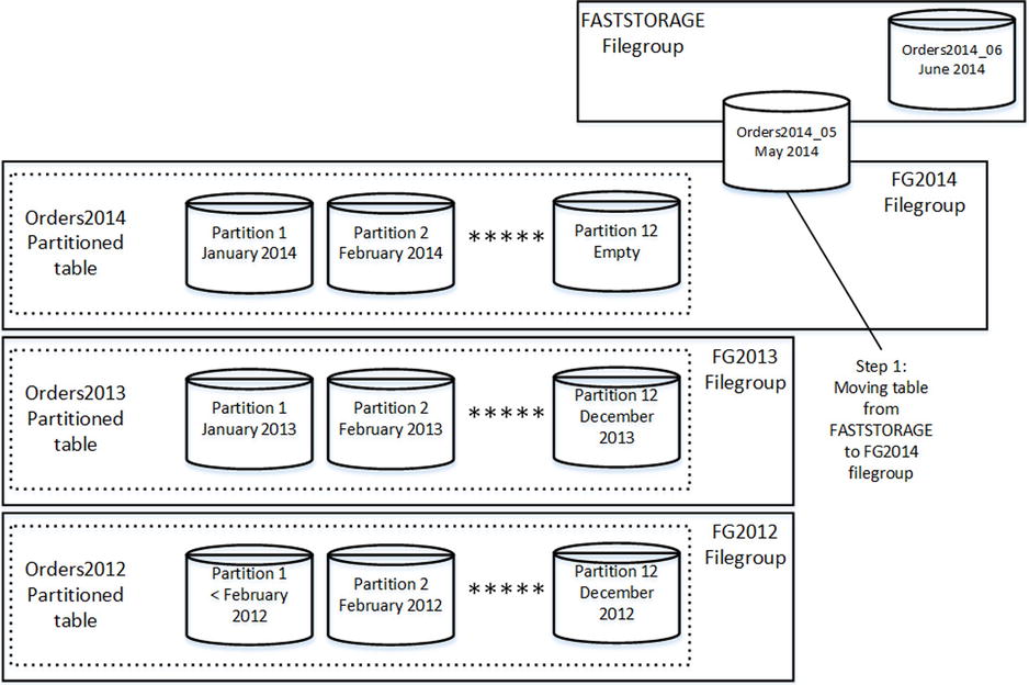
Figure 15-14. Tiered Storage in Action: Moving the Orders2014_05 table
After that, you switch the Orders2014_05 table as the partition of the Orders2014 table, creating a new Orders2014_07 table in the FASTSTORAGE filegroup and recreating the partitioned view. You can see those steps demonstrated in Figure 15-15.
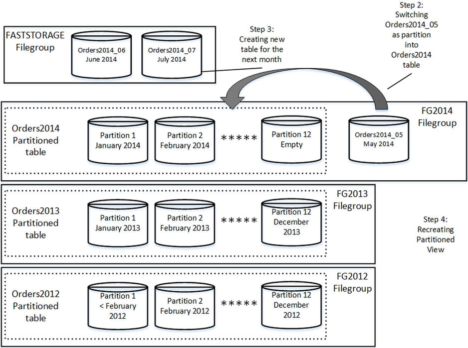
Figure 15-15. Tiered Storage in Action: Further steps
All of these operations can be done online with the Enterprise Edition of SQL Server 2012 and above. They can also be done online with SQL Server 2005-2008R2, as long as the tables do not contain LOB columns.
There is still the possibility of a lengthy hold of the schema modification (SCH-M) lock at the time when you switch Orders2014_05 into the Orders2013 table. One of the things you need to do during this process is to change the CHECK constraint on the Orders2014 table, indicating that the table now stores May 2014 data. Unfortunately, SQL Server always scans one of the indexes in the table to validate CHECK constraints and holds the schema modification (SCH-M) lock during the scan.
One of the ways to work around such a problem is to create multiple CHECK constraints at the CREATE TABLE stage and drop them later. In the example shown in Listing 15-26, we create 12 CHECK constraints in the Orders2014 table. Every time we switch the operational table as the partition, we are dropping a constraint, a metadata operation, rather than creating a new one.
Listing 15-26. Creating Multiple CHECK constraints on a table
create table dbo.Orders2014
(
        OrderId int not null,
        OrderDate datetime2(0) not null,
        OrderNum varchar(32) not null,
        OrderTotal money not null,
        CustomerId int not null,

        constraint CHK_Orders2014_01
        check(OrderDate >= '2014-01-01' and OrderDate < '2014-02-01'),

        constraint CHK_Orders2014_02
        check(OrderDate >= '2014-01-01' and OrderDate < '2014-03-01'),

        constraint CHK_Orders2014_03
        check(OrderDate >= '2014-01-01' and OrderDate < '2014-04-01'),

        constraint CHK_Orders2014_04
        check(OrderDate >= '2014-01-01' and OrderDate < '2014-05-01'),

        constraint CHK_Orders2014_05
        check(OrderDate >= '2014-01-01' and OrderDate < '2014-06-01'),

        constraint CHK_Orders2014_06
        check(OrderDate >= '2014-01-01' and OrderDate < '2014-07-01'),

        constraint CHK_Orders2014_07
        check(OrderDate >= '2014-01-01' and OrderDate < '2014-08-01'),

        constraint CHK_Orders2014_08
        check(OrderDate >= '2014-01-01' and OrderDate < '2014-09-01'),

        constraint CHK_Orders2014_09
        check(OrderDate >= '2014-01-01' and OrderDate < '2014-10-01'),

        constraint CHK_Orders2014_10
        check(OrderDate >= '2014-01-01' and OrderDate < '2014-11-01'),

        constraint CHK_Orders2014_11
        check(OrderDate >= '2014-01-01' and OrderDate < '2014-12-01'),

        constraint CHK_Orders2014
        check(OrderDate >= '2014-01-01' and OrderDate < '2015-01-01')
)
on [FG2014]
SQL Server evaluates all constraints during optimization and picks the most restrictive one.
![]() Note Even though SQL Server does not prevent you from creating hundreds or even thousands CHECK constraints per table, you should be careful about doing just that. An extremely large number of CHECK constraints slows down query optimization. Moreover, in some cases, optimization can fail due to stack size limitation. With all that being said, such an approach works fine with a non-excessive number of constraints.
Note Even though SQL Server does not prevent you from creating hundreds or even thousands CHECK constraints per table, you should be careful about doing just that. An extremely large number of CHECK constraints slows down query optimization. Moreover, in some cases, optimization can fail due to stack size limitation. With all that being said, such an approach works fine with a non-excessive number of constraints.
Tiered Storage and High Availability Technologies
Even though we will discuss High Availability (HA) Technologies in greater depth in Chapter 31, “Designing a High Availability Strategy,” it is important to mention their compatibility with Tiered Storage and data movement in this chapter. There are two different factors to consider: database files and filegroups management and data movement overhead. Neither of them affects the SQL Server Failover Cluster, where you have a single copy of the database. However, such is not the case for transaction-log based HA technologies, such as AlwaysOn Availability Groups, Database Mirroring, and Log Shipping.
Neither of the High Availability technologies prevents you from creating database files. However, with transaction-log based HA technologies, you should maintain exactly the same folder and disk structure on all nodes and SQL Server must be able to create new files in the same path everywhere. Otherwise, HA data flow would be suspended.
Another important factor is the overhead introduced by the index rebuild or DBCC SHRINKFILE commands. They are very I/O intensive and generate a huge amount of transaction log records. All of those records need to be transmitted to secondary nodes, which could saturate the network.
There is one lesser-known problem, though. Transaction-log based HA technologies work with transaction log records only. There is a set of threads, called REDO threads, which asynchronously replay transaction log records and apply changes in the data files on the secondary nodes.
![]() Note Even with synchronous synchronization, available in AlwaysOn Availability Groups and Database Mirroring, SQL Server synchronously saves (hardens) the log record in transaction logs only. The REDO threads apply changes in the database files asynchronously.
Note Even with synchronous synchronization, available in AlwaysOn Availability Groups and Database Mirroring, SQL Server synchronously saves (hardens) the log record in transaction logs only. The REDO threads apply changes in the database files asynchronously.
The performance of REDO threads is the limiting factor here. Data movement usually generates transaction log records faster than REDO threads can apply the changes in the data files. It is not uncommon for the REDO process to require minutes or even hours to catch up. This could lead to extended system downtimes in the case of failover because the database in the new primary node stays in a recovery state until the REDO stage is done.
You should also be careful if you are using readable secondaries with AlwaysOn Availability Groups. Even though the data is available during the REDO process, it is not up to date and queries against primary and secondary nodes will return different results.
![]() Note Any type of heavy transaction log activity can introduce such a problem with readable secondaries.
Note Any type of heavy transaction log activity can introduce such a problem with readable secondaries.
You should be careful implementing Tiered Storage when transaction-log based HA technologies are in use. You should factor potential downtime during failover into availability SLA and minimize it by moving data on an index-by-index basis, allowing the secondaries to catch up in between operations. You should also prevent read-only access to secondaries during data movement.
Implementing Sliding Window Scenario and Data Purge
OLTP systems often have the requirement of keeping data for a specific time. For example, an Order Entry system could keep orders for a year and have the process, which is running the first day of the every month, to delete older orders. With this implementation, called a sliding window scenario, you have a window on the data that slides and purges the oldest data, based on a given schedule.
The only way to implement a sliding window scenario with non-partitioned data is by purging the data with DELETE statements. This approach introduces huge I/O and transaction log overhead. Moreover, it could contribute to concurrency and blocking issues in the system. Fortunately, data partitioning dramatically simplifies this task, making purge a metadata-only operation.
When you implement a sliding window scenario, you usually partition the data based on the purge interval. Even though it is not a requirement, it helps you to keep the purge process on a metadata level. As an example, in the Order Entry system described above, you could partition the data on a monthly basis.
In the case of partitioned views, the purge process is simple. You need to drop the oldest table, create another table for the next partition period data, and then recreate the partitioned view. It is essential to have the next partition period data table predefined to make sure that there is always a place where the data can be inserted.
Partitioned table implementation is similar. You can purge old data by switching the corresponding partition to a temporary table, which you can truncate afterwards. For the next month’s data, you need to use the split partition function.
There is the catch, though. In order to keep the operation on a metadata level and reduce time that the schema modification (SCH-M) lock is held, you should keep the rightmost partition empty. This prevents SQL Server from moving data during the split process, which can be very time consuming in the case of large tables.
![]() Note Even metadata-level partition switch can lead to locking and blocking in very active OLTP systems. SQL Server 2014 introduces the concept of low-priority locks, which can be used to improve system concurrency during such operations. We will discuss low-priority locks in detail in Chapter 23, “Schema Locks.”
Note Even metadata-level partition switch can lead to locking and blocking in very active OLTP systems. SQL Server 2014 introduces the concept of low-priority locks, which can be used to improve system concurrency during such operations. We will discuss low-priority locks in detail in Chapter 23, “Schema Locks.”
Let’s look at an example, assuming that it is now June 2014 and the purge process will run on July 1st. As you can see in Listing 15-27, the partition function pfOrderData has boundary values of 2014-07-01 and 2014-08-01. Those values predefine two partitions: one for the July 2014 data and an empty rightmost partition that you would split during the purge process.
Listing 15-27. Sliding Window scenario: Object creation
create partition function pfOrderData(datetime2(0))
as range right for values
('2013-07-01','2013-08-01','2013-09-01','2013-10-01'
,'2013-11-01','2013-12-01','2014-01-01','2014-02-01'
,'2014-03-01','2014-04-01','2014-05-01','2014-06-01'
,'2014-07-01','2014-08-01' /* One extra empty partition */
);

create partition scheme psOrderData
as partition pfOrderData
all to ([FG1]);

create table dbo.OrderData
(
        OrderId int not null,
        OrderDate datetime2(0) not null,
        OrderNum varchar(32) not null,
        OrderTotal money not null,
        CustomerId int not null,
        /* Other Columns */
);

create unique clustered index IDX_OrderData_OrderDate_OrderId
on dbo.OrderData(OrderDate, OrderId)
on psOrderData(OrderDate);

create nonclustered index IDX_OrderData_CustomerId
on dbo.OrderData(CustomerId)
on psOrderData(OrderDate);

create table dbo.OrderDataTmp
(
        OrderId int not null,
        OrderDate datetime2(0) not null,
        OrderNum varchar(32) not null,
        OrderTotal money not null,
        CustomerId int not null,
        /* Other Columns */
);

create unique clustered index IDX_OrderDataTmp_OrderDate_OrderId
on dbo.OrderDataTmp(OrderDate, OrderId)
on [FG1];

create nonclustered index IDX_OrderDataTmp_CustomerId
on dbo.OrderDataTmp(CustomerId)
on [FG1];
It is important to have both partitions predefined. The data will be inserted into the July 2014 partition as of midnight of July 1st, before the purge process is running. The empty rightmost partition guarantees that the partition split during the purge process will be done at the metadata level.
There is also an OrderDataTmp table created in the script, which we will use as the destination for partition switch and purge. That table must reside in the same filegroup with the leftmost partition and have the same schema and indexes defined.
The purge process is shown in Listing 15-28. It switches the leftmost partition to the temporary table and splits the rightmost partition, creating a new empty partition for next month’s run.
Listing 15-28. Sliding Window scenario: Purge process
-- Purging old partition
alter table dbo.OrderData switch partition 1 to dbo.OrderDataTmp;
truncate table dbo.OrderDataTmp;

-- Creating new partition
alter partition scheme psOrderData next used [FG1];
alter partition function pfOrderData() split range('2014-09-01')
Potential Issues
Despite all of the benefits that data partitioning delivers, they do come at a cost. First, SQL Server requires a partitioned column to be a part of the clustered index key in the partitioned table. This, in turn, adds that column to the row-id and increases the row size in every nonclustered index. For example, in a table that stores 365 million rows, a datetime-partitioned column adds 2.7GB per nonclustered index, not counting fragmentation overhead and non-leaf level storage space.
![]() Tip Always choose the most storage-efficient data type based on the business requirements. In the previous example, you can use smalldatetime (4 bytes) or datetime2(0) (6 bytes) instead of datetime (8 bytes), if one minute or one second precisions are acceptable.
Tip Always choose the most storage-efficient data type based on the business requirements. In the previous example, you can use smalldatetime (4 bytes) or datetime2(0) (6 bytes) instead of datetime (8 bytes), if one minute or one second precisions are acceptable.
Even though you can mitigate this space increase in some cases by implementing data compression on the historical data, the row-id size increase can add new non-leaf levels to the indexes and extra reads when SQL Server traverses index B-Trees.
Uniqueness support is another issue. You cannot create a unique constraint and/or index on a partitioned view. With partitioned tables, SQL Server requires a partitioned column to be part of aligned unique nonclustered indexes. This enforces uniqueness only in the single partition scope. Although you can define non-aligned unique indexes, it prevents you from using a partition switch, which is one of the greatest benefits of partitioned tables.
Unfortunately, there is no easy solution for this problem. In cases where you need to support uniqueness across multiple data partitions, you have to implement complex code, often using a SERIALIZEABLE transaction isolation level, and this can introduce blocking issues in the system.
![]() Note We will discuss transaction isolation levels in greater depth in Chapter 17, “Lock Types.”
Note We will discuss transaction isolation levels in greater depth in Chapter 17, “Lock Types.”
Ultimately, the biggest problem with data partitioning is that it changes the execution plans of the queries. It can introduce suboptimal performance for some queries, which worked just fine when the data had not been partitioned.
Let’s look at one such example and create a non-partitioned table and populate it with some random data, as shown in Listing 15-29.
Listing 15-29. Potential issues with data partitioning: Creating a non-partitioned table
create table dbo.Data
(
        Id int not null,
        DateCreated datetime not null
                constraint DEF_Data_DateCreated
                default getutcdate(),
        DateModified datetime not null
                constraint DEF_Data_DateModified
                default getutcdate(),
        Placeholder char(500) null
);

create unique clustered index IDX_Data_Id
on dbo.Data(DateCreated, Id);

create unique nonclustered index IDX_Data_DateModified_Id
on dbo.Data(DateModified, Id);

declare @StartDate datetime = '2014-01-01';

;with N1(C) as (select 0 UNION ALL select 0) -- 2 rows
,N2(C) as (select 0 from N1 as T1 cross join N1 as T2) -- 4 rows
,N3(C) as (select 0 from N2 as T1 cross join N2 as T2) -- 16 rows
,N4(C) as (select 0 from N3 as T1 cross join N3 as T2) -- 256 rows
,N5(C) as (select 0 from N4 as T1 cross join N4 as T2) -- 65,536 rows
,N6(C) as (select 0 from N5 as T1 cross join N2 as T2 cross join N1 as T3)
-- 524,288 rows
,IDs(ID) as (select row_number() over (order by (select NULL)) from N6)
insert into dbo.Data(ID, DateCreated, DateModified)
        select ID, dateadd(second,35 * Id,@StartDate),
           case
                  when ID % 10 = 0
                  then dateadd(second,
                                24 * 60 * 60 * (ID % 31) + 11200 + ID % 59 + 35 * ID,
                                @StartDate)
                  else dateadd(second,35 * ID,@StartDate)
           end
        from IDs;
Let's assume that we have a process that reads modified data from the table and exports it somewhere. While there are a few different ways to implement such a task, perhaps the simplest method is to use a query, as shown in Listing 15-30, with the @DateModified parameter representing the most recent DateModified value from the previous record set read.
Listing 15-30. Potential issues with data partitioning: Reading modified data
select top (@Top) Id, DateCreated, DateModified, PlaceHolder
from dbo.Data
where DateModified > @LastDateModified
order by DateModified, Id
The execution plan of the query, which selects 100 rows, is shown in Figure 15-16. The plan is very efficient, and it utilizes a Nonclustered Index Seek with range scan. SQL Server finds the first row with a DateModified value that exceeds @LastDateModified and then scans the index selecting the first 100 rows from there.
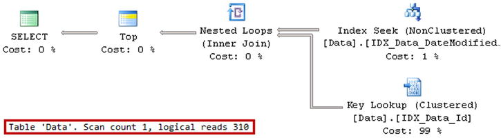
Figure 15-16. Execution plan with non-partitioned table
Now let’s partition the table on a monthly basis, as shown in Listing 15-31.
Listing 15-31. Potential issues with data partitioning: Partitioning the table
create partition function pfData(datetime)
as range right for values
('2014-02-01', '2014-03-01','2014-04-01','2014-05-01'
,'2014-06-01','2014-07-01','2014-08-01'),

create partition scheme psData
as partition pfData
all to ([FG1]);

create unique clustered index IDX_Data_DateCreated_Id
on dbo.Data(DateCreated,ID)
on psData(DateCreated);

create unique nonclustered index IDX_Data_DateModified_Id_DateCreated
on dbo.Data(DateModified, ID, DateCreated)
on psData(DateCreated);
If you run the code from Listing 15-30 again, the execution plan would change as shown in Figure 15-17. As you can see, SQL Server decides to use a Clustered Index Scan, which dramatically decreases the performance of the query.
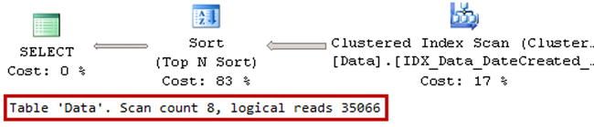
Figure 15-17. Execution plan with partitioned table
The root cause of the problem is related to the fact that the data in clustered and nonclustered indexes are now sorted on a partition-by-partition basis rather than across the entire table. You can think about each partition as an individual table with its own set of data and indexes. SQL Server decides that, in such a situation, a clustered index scan is the cheapest option with which to proceed.
Let's look what happens if you force SQL Server to use a nonclustered index with an index hint, as shown in Listing 15-32.
Listing 15-32. Potential issues with data partitioning: Using a nonclustered index with a hint
declare
        @LastDateModified datetime = '2014-05-25'

select top 100 Id, DateCreated, DateModified, PlaceHolder
from dbo.Data with (index=IDX_Data_DateModified_Id_DateCreated)
where DateModified > @LastDateModified
order by DateModified, Id
As you can see in Figure 15-18, the execution plan is even less efficient than before. SQL Server located and read all of the rows with a DateModified greater than @LastDateModified from every partition, and it performed a Key Lookup operation for all of them, sorting the data afterwards.

Figure 15-18. Execution plan with index hint
There is no easy way to fix the problem. You can use non-aligned nonclustered indexes, which are not partitioned. Unfortunately, you cannot use a partition switch in such cases nor perform piecemeal database restore, making subsets of the data available to customers. Thus the only option you have is code refactoring.
![]() Tip You can drop a non-aligned nonclustered index before a partition switch and recreate it after the switch is done.
Tip You can drop a non-aligned nonclustered index before a partition switch and recreate it after the switch is done.
The $PARTITION system function returns a partition number for the value provided as a parameter. You can use this function in a where clause in the query, which eliminates other partitions and produces execution plans similar to the queries against non-partitioned tables. You can see the query, which reads modified rows from partition 5, in Listing 15-33.
Listing 15-33. Potential issues with data partitioning: Selecting data from the single partition
declare
        @LastDateModified datetime = '2014-05-25'

select top 100 Id, DateCreated, DateModified, PlaceHolder
from dbo.Data with (index=IDX_Data_DateModified_Id_DateCreated)
where
        DateModified > @LastDateModified and
        $partition.pfData(DateCreated) = 5
order by DateModified, Id
As you can see in Figure 15-19, the execution plan is very similar to the query that read modified data from the non-partitioned table.

Figure 15-19. Execution plan for the query: selecting data from the single partition
In some cases, you can use this behavior to optimize queries against partitioned tables. In our case, you can have the following algorithm:
- Read the top 100 modified rows from every partition using the $PARTITION function, limiting execution to the single partition scope.
- Sort rows read in the previous step, and select the top 100 rows across all partitions.
- Select data from the clustered index for the 100 rows returned by the previous step.
The first step of the algorithm requires you to know the number of partitions in the table. You can use sys.partition_range_values DMV to find the number of boundary values in the partition function, which is one less than the number of partitions in the table.
The code in Listing 15-34 shows an optimized version of the query. Partitions CTE returns the numbers that correspond to the partition numbers in the table, which are used as filters in the CROSS APPLY operator of Steps1and2 CTE. The CROSS APPLY operator implements the first step of the algorithm. Select in CROSS APPLY executed once per partition.
Listing 15-34. Potential issues with data partitioning: Optimized query
declare
        @LastDateModified datetime = '2014-05-25'
        ,@BoundaryValuesCount int

-- Getting number of boundary values in partition function
select @BoundaryValuesCount = max(boundary_id)
from sys.partition_functions pf join
        sys.partition_range_values prf on
                pf.function_id = prf.function_id
where pf.name = 'pfData'

;with Partitions(PartitionNum)
as
(
        select 1
        union all
        select PartitionNum + 1
        from Partitions
        where PartitionNum <= @BoundaryValuesCount
)
,Steps1and2(Id, DateCreated, DateModified)
as
(
        select top 100 PartData.ID, PartData.DateCreated, PartData.DateModified
        from Partitions p
                cross apply
                ( -- Step 1 - runs once per partition
                        select top 100 Id, DateCreated, DateModified
                        from dbo.Data
                        where
                                DateModified > @LastDateModified and
                                $Partition.pfData(DateCreated) =
                                        p.PartitionNum
                        order by DateModified, ID
                ) PartData
        order by PartData.DateModified, PartData.Id
)
-- Step 3 - CI seek as Key Lookup operation
select s.Id, s.DateCreated, s.DateModified, d.Placeholder
from Steps1and2 s join dbo.Data d on
        d.Id = s.Id and s.DateCreated = d.DateCreated
order by s.DateModified, s.Id
The outer select statement in Steps1and2 CTE sorts the data returned by the CROSS APPLY operator across all partitions, which is the second step in the algorithm.
Finally, the last select outside of CTE is the third step in the algorithm described above.
You can see the execution plan of the query in Figure 15-20. The plan is almost as efficient as the one against non-partitioned tables.

Figure 15-20. Execution plan of the optimized query
Unfortunately, SQL Server underestimates the number of executions and rows returned by recursive CTE. It can lead to further cardinality estimation errors and subefficient execution plans in some cases. You can avoid this error by using a temporary table to store partition numbers, as shown in Listing 15-35.
Listing 15-35. Storing partition numbers in a temporary table
declare
        @LastDateModified datetime = '2014-05-25',
        @BoundaryValuesCount int

create table #Partitions(PartitionNum smallint not null);

-- Getting number of boundary values in partition function
select @BoundaryValuesCount = max(boundary_id)
from sys.partition_functions pf join
        sys.partition_range_values prf on
                pf.function_id = prf.function_id
where pf.name = 'pfData'

;with Partitions(PartitionNum)
as
(
        select 1
        union all
        select PartitionNum + 1
        from Partitions
        where PartitionNum <= @BoundaryValuesCount
)
insert into #Partitions(PartitionNum)
        select PartitionNum from Partitions;

;with Steps1and2(Id, DateCreated, DateModified)
as
(
        select top 100 PartData.ID, PartData.DateCreated, PartData.DateModified
        from #Partitions p
                cross apply
                (
                        select top 100 Id, DateCreated, DateModified
                        from dbo.Data
                        where
                                DateModified > @LastDateModified and
                                $Partition.pfData(DateCreated) =
                                        p.PartitionNum
                        order by DateModified, ID
                ) PartData
        order by PartData.DateModified, PartData.Id
)
-- Step 3 - CI seek as Key Lookup operation
select s.Id, s.DateCreated, s.DateModified, d.Placeholder
from Steps1and2 s join dbo.Data d on
        d.Id = s.Id and s.DateCreated = d.DateCreated
order by s.DateModified, s.Id
Alternatively, if the number of partitions is static and predefined, you can hardcode it in Partitions CTE, as shown in Listing 15-36.
Listing 15-36. Hardcoding partition numbers
declare
        @LastDateModified datetime = '2014-05-25'

;with Partitions(PartitionNum)
as
(
        select v.V
        from (values(1),(2),(3),(4),(5),(6),(7),(8)) v(V)
)
,Steps1and2(Id, DateCreated, DateModified)
as
(
        select top 100 PartData.ID, PartData.DateCreated, PartData.DateModified
        from Partitions p
                cross apply
                (
                        select top 100 Id, DateCreated, DateModified
                        from dbo.Data
                        where
                                DateModified > @LastDateModified and
                                $Partition.pfData(DateCreated) =
                                        p.PartitionNum
                        order by DateModified, ID
                ) PartData
        order by PartData.DateModified, PartData.Id
)
-- Step 3 - CI seek as Key Lookup operation
select s.Id, s.DateCreated, s.DateModified, d.Placeholder
from Steps1and2 s join dbo.Data d on
        d.Id = s.Id and s.DateCreated = d.DateCreated
order by s.DateModified, s.Id
To repeat, data partitioning changes the execution plans of the queries. You should carefully test systems in a staging environment using databases of similar size and data distribution to that of production. This will help to avoid unpleasant surprises when changes are implemented on production servers.
Summary
Management of a large amount of data is a challenging task, especially when the data is not partitioned. Keeping a large amount of data in the same place is not efficient for several different reasons. It increases storage costs and introduces overhead due to the different workload and index management requirements for the various parts of the data. Moreover, it prevents piecemeal database restore, which complicates availability SLA compliance.
There are two main data partitioning techniques available in SQL Server. Partitioned tables are available in the Enterprise Edition of SQL Server. They allow you to partition table data into separate internal tables/partitions, which is transparent to client applications. Each partition can be placed in its own filegroup and have its own data compression. However, the database schema, indexes, and statistics are the same across all partitions.
Alternatively, you can partition the data by separating it between multiple tables, combining all of them through a partitioned view using the union all operator. Every table can have its own schema and set of indexes and maintain its own statistics. Partitioned views are supported in all editions of SQL Server.
Although partitioned views are more flexible, such an implementation requires code refactoring and increases the system maintenance cost due to the large number of tables involved. You can reduce that cost by combining both partitioned tables and views together.
Data partitioning helps reduce storage subsystem cost by implementing tiered storage. With such an approach, you can place active operational data on a fast disk array while keeping old, rarely accessed historical data on cheaper disks. You should design a strategy that allows you to move data between different disk arrays when needed. Different versions and editions of SQL Server require different implementation approaches for this task.
You should be careful when moving a large amount of data when transaction-log based High Availability technologies are in use. A large amount of transaction log records leads to REDO process backlog on secondary nodes and can increase system downtime in case of a failover. Moreover, you should prevent queries from accessing readable secondaries in case of a backlog.
You can use data partitioning to improve the performance and concurrency of data import and purge operations. Make sure to keep the rightmost partition empty when you are implementing a sliding window scenario in the system.
Finally, data partitioning comes at a cost. In the case of partitioned tables, a partition column must be included in the clustered index, which increases the size of nonclustered index rows. Moreover, indexes are sorted within individual partitions. This can lead to suboptimal execution plans and regressions after partitioning has been implemented. The $PARTITION function can be used to access data in individual partitions, and this can help with optimization.