![]()
SQL Server Query Optimizer uses a cost-based model when choosing an execution plan for queries. It estimates the cost of the different execution plans and chooses the one with the lowest cost. Remember, however, that SQL Server does not search for the best execution plan available for the query, as evaluating all possible alternatives is time consuming and expensive in terms of the CPU. The goal of Query Optimizer is finding a good enough execution plan, fast enough.
Cardinality estimation (estimation of the number of rows that need to be processed on each step of the query execution) is one of the most important factors in query optimization. This number affects the choice of join strategies; amount of memory (memory grant) required for query execution, and quite a few other things.
The choice of indexes to use while accessing the data is among those factors. As you will remember, Key and RID Lookup operations are expensive in terms of I/O, and SQL Server does not use nonclustered indexes when it estimates that a large number of Key or RID Lookup operations will be required. SQL Server maintains the statistics on indexes and, in some cases on columns, which help in performing such estimations.
Introduction to SQL Server Statistics
SQL Server statistics are the system objects that contain the information about data distribution in the index key values and, sometimes, regular column values. Statistics can be created on any data type that supports comparison operations, such as >, <, =, and so on.
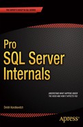
Let’s examine the IDX_BOOKS_ISBN index statistics from the dbo.Books table we created in Listing 2-15 in the previous chapter. You can do this by using DBCC SHOW_STATISTICS ('dbo.Books',IDX_BOOKS_ISBN) command. The results are shown in Figure 3-1.
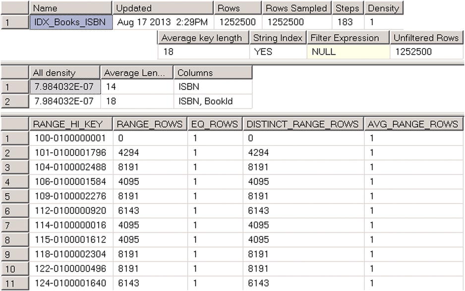
Figure 3-1. DBCC SHOW_STATISTICS output
As you can see, the DBCC SHOW_STATISTICS command returns three result sets. The first one contains general metadata information about statistics, such as name, update date, number of rows in the index at the time when the statistics were updated, and so on. The Steps column in the first result set indicates the number of steps/values in the histogram (more about this later). Density is calculated based on the formula: 1 / frequency, where frequency indicates the average number of the duplicates per key value. The query optimizer does not use this value, and it is displayed for backwards-compatibility purposes only.
The second result set contains information about density for the combination of key values from the statistics (index). It is calculated based on 1 / number of distinct values formula, and it indicates how many rows on average every combination of key values has. Even though the IDX_Books_ISBN index has just one key column ISBN defined, it also includes a clustered index key as part of the index row. Our table has 1,252,500 unique ISBN values, and the density for the ISBN column is 1.0 / 1,252,500 = 7.984032E-07. All combinations of (ISBN, BookId) columns are also unique and have the same density.
The last result set is called the histogram. Every record in the histogram, called a histogram step, includes the sample key value from the leftmost column from the statistics (index) and information about the data distribution in the range of values from the preceding to the current RANGE_HI_KEY value. Let’s examine histogram columns in greater depth.
- The RANGE_HI_KEY column stores the sample value of the key. This value is the upper-bound key value for the range defined by histogram step. For example, record (step) #3 with RANGE_HI_KEY = '104-0100002488' in the histogram from Figure 3-1 stores information about the interval of: ISBN > '101-0100001796' and ISBN <= '104-0100002488'.
- The RANGE_ROWS column estimates the number of rows within the interval. In our case, the interval defined by record (step) #3 has 8,191 rows.
- EQ_ROWS indicates how many rows have a key value equal to the RANGE_HI_KEY upper-bound value. In our case, there is only one row with ISBN = '104-0100002488'.
- DISTINCT_RANGE_ROWS indicates how many distinct values of the keys are within the interval. In our case, all of the values of the keys are unique and DISTINCT_RANGE_ROWS = RANGE_ROWS.
- AVG_RANGE_ROWS indicates the average number of rows per distinct key value in the interval. In our case, all of the values of the keys are unique and AVG_RANGE_ROWS = 1.
Let’s insert a set of the duplicate ISBN values into the index with the code shown in Listing 3-1.
Listing 3-1. Inserting duplicate ISBN values into the index
;with Prefix(Prefix)
as
(
        select Num
        from (values(104),(104),(104),(104),(104)) Num(Num)

)
,Postfix(Postfix)
as
(
        select 100000001
        union all
        select Postfix + 1
        from Postfix
        where Postfix < 100002500
)
insert into dbo.Books(ISBN, Title)
        select
                CONVERT(char(3), Prefix) + '-0' + CONVERT(char(9),Postfix)
                ,'Title for ISBN' + CONVERT(char(3), Prefix) + '-0' + CONVERT(char(9),Postfix)
        from Prefix cross join Postfix
option (maxrecursion 0);

-- Updating the statistics
update statistics dbo.Books IDX_Books_ISBN with fullscan;
Now, if you run the DBCC SHOW_STATISTICS ('dbo.Books',IDX_BOOKS_ISBN) command again, you will see the results shown in Figure 3-2.
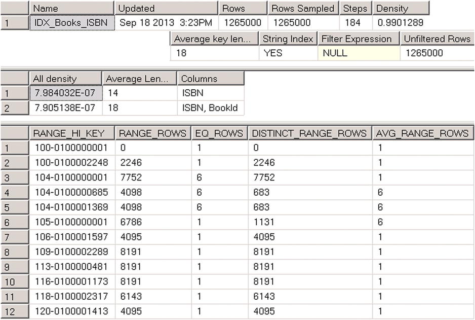
Figure 3-2. DBCC SHOW_STATISTICS output
ISBN values with the prefix 104 now have the duplicates, and this affects the histogram. It is also worth mentioning that the density information in the second result set is also changed. The density for ISBNs with duplicate values is higher than for the combination of (ISBN, BookId) columns, which is still unique.
Let’s run the query shown in Listing 3-2, and check the execution plan, as shown in Figure 3-3.
Listing 3-2. Selecting data for ISBNs starting with ‘114’
select BookId, ISBN, Title from dbo.Books where ISBN like '114%'

Figure 3-3. Execution plan of the query
There are two important properties that most execution plan operators have. Actual Number of Rows indicates how many rows were processed during query execution. Estimated Number of Rows indicates the number of rows SQL Server estimated during the Query Optimization stage. In our case, SQL Server estimates that there are 2,625 rows with ISBNs starting with ‘114’. If you look at the histogram shown in Figure 3-2, you will see that step 10 stores the information about the data distribution for the ISBN interval that includes the values that you are selecting. Even with linear approximation, you can estimate the number of rows close to what SQL Server determined.
![]() Note SQL Server stores additional information in the statistics for the string values called Trie Trees. This allows SQL Server to perform better cardinality estimation in the case of string keys. This feature is not documented, and it is outside of the scope of the book.
Note SQL Server stores additional information in the statistics for the string values called Trie Trees. This allows SQL Server to perform better cardinality estimation in the case of string keys. This feature is not documented, and it is outside of the scope of the book.
There are two very important things to remember about statistics.
- The histogram stores information about data distribution for the leftmost statistics (index) column only. There is information about the multi-column density of the key values in statistics, but that is it. All other information in the histogram relates to data distribution for the leftmost statistics column only.
- SQL Server retains at most 200 steps in the histogram, regardless of the size of the table. The intervals covered by each histogram step increase as the table grows. This leads to less accurate statistics in the case of large tables.
![]() Tip In the case of composite indexes, when all columns from the index are used as predicates in all queries, it is beneficial to define a column with lower density/higher selectivity as the leftmost column of the index. This will allow SQL Server to better utilize the data distribution information from the statistics.
Tip In the case of composite indexes, when all columns from the index are used as predicates in all queries, it is beneficial to define a column with lower density/higher selectivity as the leftmost column of the index. This will allow SQL Server to better utilize the data distribution information from the statistics.
You should consider the SARGability of the predicates, however. For example, if all queries are using FirstName=@FirstName and LastName=@LastName predicates in the where clause, it is better to have LastName as the leftmost column in the index. Nonetheless, this is not the case for predicates like FirstName=@FirstName and LastName<>@LastName, where LastName is not SARGable.
Index selectivity is a metric, which is the opposite of density. It is calculated based on the formula 1 / density. The more unique values a column has, the higher its selectivity.
![]() Note We will talk about index design considerations in greater detail in Chapter 6, “Designing and Tuning the Indexes.”
Note We will talk about index design considerations in greater detail in Chapter 6, “Designing and Tuning the Indexes.”
Column-Level Statistics
In addition to index-level statistics, you can create separate column-level statistics. Moreover, in some cases, SQL Server creates such statistics automatically.
Let’s take a look at an example and create a table and populate it with the data shown in Listing 3-3.
Listing 3-3. Column-level statistics: Table creation
create table dbo.Customers
(
        CustomerId int not null identity(1,1),
        FirstName  nvarchar(64) not null,
        LastName nvarchar(128) not null,
        Phone varchar(32) null,
        Placeholder char(200) null
);

create unique clustered index IDX_Customers_CustomerId
on dbo.Customers(CustomerId)
go

-- Inserting cross-joined data for all first and last names 50 times
-- using GO 50 command in Management Studio
;with FirstNames(FirstName)
as
(
        select Names.Name
        from
        (
                values('Andrew'),('Andy'),('Anton'),('Ashley'),('Boris'),
                ('Brian'),('Cristopher'),('Cathy'),('Daniel'),('Donny'),
                ('Edward'),('Eddy'),('Emy'),('Frank'),('George'),('Harry'),
                ('Henry'),('Ida'),('John'),('Jimmy'),('Jenny'),('Jack'),
                ('Kathy'),('Kim'),('Larry'),('Mary'),('Max'),('Nancy'),
                ('Olivia'),('Olga'),('Peter'),('Patrick'),('Robert'),
                ('Ron'),('Steve'),('Shawn'),('Tom'),('Timothy'),
                ('Uri'),('Vincent')
        ) Names(Name)
)
,LastNames(LastName)
as
(
        select Names.Name
        from
        (
                values('Smith'),('Johnson'),('Williams'),('Jones'),('Brown'),
                        ('Davis'),('Miller'),('Wilson'),('Moore'),('Taylor'),
                        ('Anderson'),('Jackson'),('White'),('Harris')
        ) Names(Name)
)
insert into dbo.Customers(LastName, FirstName)
        select LastName, FirstName
        from FirstNames cross join LastNames
go 50

insert into dbo.Customers(LastName, FirstName) values('Isakov','Victor')
go

create nonclustered index IDX_Customers_LastName_FirstName
on dbo.Customers(LastName, FirstName);
Every combination of first and last names specified in the first insert statement has been inserted into the table 50 times. In addition, there is one row, with the first name Victor, inserted by the second insert statement.
Now let’s assume that you want to run the query that selects the data based on the FirstName parameter only. That predicate is not SARGable for the IDX_Customers_LastName_FirstName index because there is no SARGable predicate on the LastName column, which is the leftmost column in the index.
SQL Server offers two different options on how to execute the query. The first option is to perform a Clustered Index Scan. The second option is to use a Nonclustered Index Scan doing Key Lookup for every row of the nonclustered index where the FirstName value matches the parameter.
The nonclustered index row size is much smaller than that of the clustered index. It uses less data pages, and a scan of the nonclustered index would be more efficient as compared to a clustered index scan, owing to the fewer I/O reads that it performs. At the same time, the plan with a nonclustered index scan would be less efficient than a clustered index scan when the table has a large number of rows with a particular FirstName and a large number of key lookups is required. Unfortunately, the histogram for the IDX_Customers_LastName_FirstName index stores the data distribution for the LastName column only, and SQL Server does not know about the FirstName data distribution.
Let’s run the two selects shown in Listing 3-4 and examine the execution plans in Figure 3-4.
Listing 3-4. Column-level statistics: Querying data
select CustomerId, FirstName, LastName, Phone
from dbo.Customers
where FirstName = 'Brian';

select CustomerId, FirstName, LastName, Phone
from dbo.Customers
where FirstName = 'Victor';

Figure 3-4. Column-level statistics: Execution plans
As you can see, SQL Server decides to use a clustered index scan for the first select, which returns 700 rows, and a nonclustered index scan for the second select, which returns a single row.
Now let’s query the sys.stats catalog view and check the table’s statistics. The code for this is shown in Listing 3-5.
Listing 3-5. Column-level statistics: Querying sys.stats view
select  stats_id, name, auto_created
from sys.stats
where object_id = object_id(N'dbo.Customers')
![]() Note Each table in Object Explorer in Management Studio has a Statistics node that shows the statistics defined in the table.
Note Each table in Object Explorer in Management Studio has a Statistics node that shows the statistics defined in the table.
The query returned three rows, as shown in Figure 3-5.
Figure 3-5. Column-level statistics: Result of the query
The first two rows correspond to the clustered and nonclustered indexes from the table. The last one, with the name that starts with the _WA prefix, displays column-level statistics, which was created automatically when SQL Server optimized our queries.
Let’s examine it with the DBCC SHOW_STATISTICS ('dbo.Customers', _WA_Sys_00000002_276EDEB3) command. As you can see in Figure 3-6, it stores information about the data distribution for the FirstName column. As a result, SQL Server can estimate the number of rows for first names, which we used as parameters, and generate different execution plans for each parameter value.
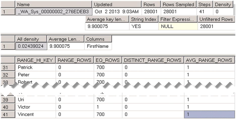
Figure 3-6. Column-level statistics: Auto-created statistics on the FirstName column
You can manually create statistics on a column or multiple columns with the CREATE STATISTICS command. Statistics created on multiple columns are similar to statistics created on composite indexes. They include information about multi-column density, although the histogram retains data distribution information for the leftmost column only.
There is overhead associated with column-level statistics maintenance, although it is much smaller than that of the index, which needs to be updated every time data modifications occur. In some cases, when particular queries do not run very often, you can elect to create column-level statistics rather than an index. Column-level statistics help Query Optimizer find better execution plans, even though those execution plans are suboptimal due to the index scans involved. At the same time, statistics do not add an overhead during data modification operations, and they help avoid index maintenance. This approach works only for rarely executed queries, however. You need to create indexes to optimize queries that run often.
Statistics and Execution Plans
SQL Server creates and updates statistics automatically by default. There are two options on the database level that control such behavior:
- Auto Create Statistics controls whether or not optimizer creates column-level statistics automatically. This option does not affect index-level statistics, which are always created. The Auto Create Statistics database option is enabled by default.
- When the Auto Update Statistics database option is enabled, SQL Server checks if statistics are outdated every time it compiles or executes a query and updates them if needed. The Auto Update Statistics database option is also enabled by default.
![]() Tip You can control statistics auto update behavior on the index level by using the STATISTICS_NORECOMPUTE index option. By default, this option is set to OFF, which means that statistics are automatically updated. Another way to change auto update behavior at the index or table level is by using the sp_autostats system stored procedure.
Tip You can control statistics auto update behavior on the index level by using the STATISTICS_NORECOMPUTE index option. By default, this option is set to OFF, which means that statistics are automatically updated. Another way to change auto update behavior at the index or table level is by using the sp_autostats system stored procedure.
SQL Server determines if statistics are outdated based on the number of changes that affect the statistics columns performed by the INSERT, UPDATE, DELETE, and MERGE statements. There are three different cases, called statistics update thresholds,also sometimes known as statistics recompilation thresholds, when SQL Server marks statistics as outdated.
- When a table is empty, SQL Server outdates statistics when you add data to an empty table.
- When a table has less than 500 rows, SQL Server outdates statistics after every 500 changes of the statistics columns.
- When a table has 500 or more rows, SQL Server outdates statistics after every 500 + (20% of total number of rows in the table) changes of the statistics columns.
It is also worth mentioning that SQL Server counts how many times the statistics columns were changed, rather than the number of changed rows. For example, if you change the same row 100 times, it would be counted as 100 changes rather than as 1 change.
That leads us to a very important conclusion. The number of changes to statistics columns required to trigger a statistics update is proportional to the table size. The larger the table, the less often statistics are automatically updated. For example, in the case of a table with 1 billion rows, you would need to perform about 200 million changes to statistics columns to make the statistics outdated. Let’s look how that behavior affects our systems and execution plans.
![]() Note SQL Server 2014 introduces a new cardinality estimation model, which changes cardinality estimations for the case shown below. We will talk about it in detail later in the chapter.
Note SQL Server 2014 introduces a new cardinality estimation model, which changes cardinality estimations for the case shown below. We will talk about it in detail later in the chapter.
At this point, the table dbo.Books has 1,265,000 rows. Let’s add 250,000 rows to the table with the prefix 999, as shown in Listing 3-6.
Listing 3-6. Adding rows to dbo.Books
;with Postfix(Postfix)
as
(
        select 100000001
        union all
        select Postfix + 1
        from Postfix
        where Postfix < 100250000
)
insert into dbo.Books(ISBN, Title)
        select
                '999-0' + CONVERT(char(9),Postfix)
                ,'Title for ISBN 999-0' + CONVERT(char(9),Postfix)
        from Postfix
option (maxrecursion 0)
Now let’s run the query that selects all of the rows with such a prefix. The query is shown in Listing 3-7.
Listing 3-7. Selecting rows with prefix 999
select * from dbo.Books where ISBN like '999%' -- 250,000 rows
If you examine the execution plan of the query shown in Figure 3-7, you will see Nonclustered Index Seek and Key Lookup operations, even though they are inefficient in cases where you need to select almost 20 percent of the rows from the table.
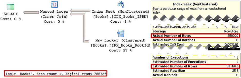
Figure 3-7. Execution plan for the query selecting rows with the 999 prefix
You will also notice in Figure 3-7 a huge discrepancy between the estimated and actual number of rows for the index seek operator. SQL Server estimated that there are only 31.4 rows with prefix 999 in the table, even though there are 250,000 rows with such a prefix. As a result, a highly inefficient plan is generated.
Let’s look at the IDX_BOOKS_ISBN statistics by running the DBCC SHOW_STATISTICS ('dbo.Books',IDX_BOOKS_ISBN) command. The output is shown in Figure 3-8. As you can see, even though we inserted 250,000 rows into the table, statistics were not updated and there is no data in the histogram for the prefix 999. The number of rows in the first result set corresponds to the number of rows in the table during the last statistics update. It does not include the 250,000 rows you inserted.

Figure 3-8. IDX_BOOKS_ISBN Statistics
Let’s update statistics using the update statistics dbo.Books IDX_Books_ISBN with fullscan command, and run the select from Listing 3-7 again. The execution plan for the query is shown in Figure 3-9. The estimated number of rows is now correct, and SQL Server ended up with a much more efficient execution plan that uses a clustered index scan with about 17 times fewer I/O reads than before.
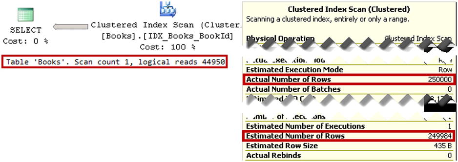
Figure 3-9. Execution plan for the query selecting rows with the 999 prefix after a statistics update
As you can see, incorrect cardinality estimations can lead to highly inefficient execution plans. Outdated statistics are, perhaps, one of the most common reasons for incorrect cardinality estimations. You can pinpoint some of these cases by examining the estimated and actual number of rows in the execution plans. The big discrepancy between these two values often indicates that statistics are incorrect. Updating statistics can solve this problem and generate more efficient execution plans.
Statistics and Query Memory Grants
SQL Server queries need memory for execution. Different operators in the execution plans have different memory requirements. Some of them do not need a lot of memory. For example, the Index Scan operator fetches rows one by one and does not need to store multiple rows in memory. Other operators, for example the Sort operator, need access to the entire rowset before it starts execution.
SQL Server tries to estimate the amount of memory (memory grant) required for a query and its operators based on row size and cardinality estimation. It is important that the memory grant is correct. Underestimations and overestimations both introduce inefficiencies. Overestimations waste SQL Server memory. Moreover, it may take longer to allocate a large memory grant on busy servers.
Underestimations, on the other hand, can lead to a situation where some operators in the execution plan do not have enough memory. If the Sort operator does not have enough memory for an in-memory sort, SQL Server spills the rowset to tempdb and sorts the data there. A similar situation occurs with hash tables. SQL Server uses tempdb if needed. In either case, using tempdb can significantly decrease the performance of an operation and a query in general.
Let’s look at an example and create a table and populate it with some data. Listing 3-8 creates the table dbo.MemoryGrantDemo and populates it with 65,536 rows. The Col column stores the values from 0 to 99, with either 655 or 656 rows per value. There is a nonclustered index on the Col column, which is created at the end of the script. As a result, statistics on that index are accurate, and SQL Server would be able to estimate correctly the number of rows per each Col value in the table.
Listing 3-8. Cardinality Estimation and Memory Grants: Table creation
create table dbo.MemoryGrantDemo
(
        ID int not null,
        Col int not null,
        Placeholder char(8000)
);

create unique clustered index IDX_MemoryGrantDemo_ID
on dbo.MemoryGrantDemo(ID);

;with N1(C) as (select 0 union all select 0) -- 2 rows
,N2(C) as (select 0 from N1 as T1 CROSS JOIN N1 as T2) -- 4 rows
,N3(C) as (select 0 from N2 as T1 CROSS JOIN N2 as T2) -- 16 rows
,N4(C) as (select 0 from N3 as T1 CROSS JOIN N3 as T2) -- 256 rows
,N5(C) as (select 0 from N4 as T1 CROSS JOIN N4 as T2) -- 65,536 rows
,IDs(ID) as (select row_number() over (order by (select NULL)) from N5)
insert into dbo.MemoryGrantDemo(ID,Col,Placeholder)
        select ID, ID % 100, convert(char(100),ID)
        from IDs;

create nonclustered index IDX_MemoryGrantDemo_Col
on dbo.MemoryGrantDemo(Col);
As a next step, shown in Listing 3-9, we add 656 new rows to the table with Col=1000. This is just 1 percent of the total table data and, as a result, the statistics are not going to be outdated. As you already know, the histogram would not have any information about the Col=1000 value.
Listing 3-9. Cardinality Estimation and Memory Grants: Adding 656 rows
;with N1(C) as (select 0 union all select 0) -- 2 rows
,N2(C) as (select 0 from N1 as T1 CROSS JOIN N1 as T2) -- 4 rows
,N3(C) as (select 0 from N2 as T1 CROSS JOIN N2 as T2) -- 16 rows
,N4(C) as (select 0 from N3 as T1 CROSS JOIN N3 as T2) -- 256 rows
,N5(C) as (select 0 from N4 as T1 CROSS JOIN N2 as T2) -- 1,024 rows
,IDs(ID) as (select row_number() over (order by (select NULL)) from N5)
insert into dbo.MemoryGrantDemo(ID,Col,Placeholder)
        select 100000 + ID, 1000, convert(char(100),ID)
        from IDs
        where ID <= 656;
Now let’s try to run two queries that select data with the predicate on the Col column using the execution plan with a Sort operator. The code for doing this is shown in Listing 3-10. I am using a variable as a way to suppress the result set from being returned to the client.
Listing 3-10. Cardinality Estimation and Memory Grants: Selecting data
declare
        @Dummy int

set statistics time on
select @Dummy = ID from dbo.MemoryGrantDemo where Col = 1 order by Placeholder
select @Dummy = ID from dbo.MemoryGrantDemo where Col = 1000 order by Placeholder
set statistics time off
Query optimizer will be able to estimate correctly the number of rows with Col=1. However, this is not the case for the Col=1000 predicate. Look at the execution plans shown in Figure 3-10.
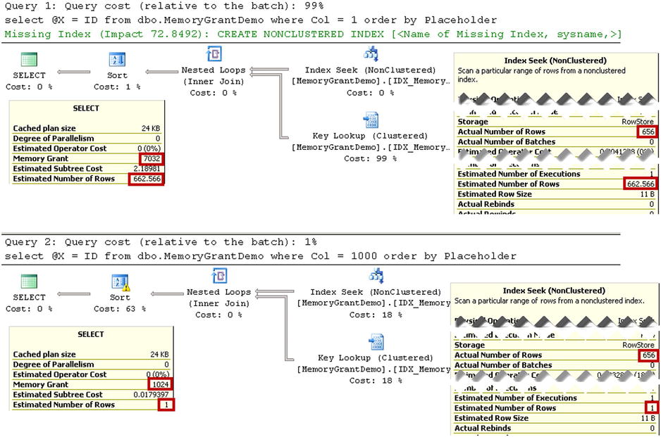
Figure 3-10. Cardinality Estimation and Memory Grants: Execution plans
Even though the execution plans look very similar, the cardinality estimations and memory grants are different. Another difference is that the Sort operator icon in the second query has an exclamation mark. If you look at the operator properties, you will see a warning, as shown in Figure 3-11. It shows that this operation spilled to tempdb.

Figure 3-11. Cardinality Estimation and Memory Grants: Sort Warning
![]() Note The new Cardinality Estimator introduced in SQL Server 2014 uses a different algorithm when estimating cardinality for values outside of the histogram. We will discuss this later in the chapter.
Note The new Cardinality Estimator introduced in SQL Server 2014 uses a different algorithm when estimating cardinality for values outside of the histogram. We will discuss this later in the chapter.
The execution time of the queries on my computer is as follows:
SQL Server Execution Times:
   CPU time = 0 ms,  elapsed time = 17 ms.

SQL Server Execution Times:
   CPU time = 16 ms,  elapsed time = 88 ms.
As you can see, the second query with the incorrect memory grant and tempdb spill is about five times slower than the first one, which performs an in-memory sort.
![]() Note You can monitor tempdb spills with SQL Profiler by capturing the Sort Warning and Hash Warning events.
Note You can monitor tempdb spills with SQL Profiler by capturing the Sort Warning and Hash Warning events.
Statistics Maintenance
As I already mentioned, SQL Server updates statistics automatically by default. This behavior is usually acceptable for small tables; however, you should not rely on automatic statistics updates in the case of large tables with millions or billions of rows. The number of changes that triggers a statistics update would be very high and, as a result, it would not be triggered often enough.
It is recommended that you update statistics manually in the case of large tables. You must analyze the size of the table, data modification patterns, and system availability when picking an optimal statistics maintenance strategy. For example, you can decide to update statistics on critical tables on a nightly basis if the system does not have a heavy load outside of business hours.
![]() Note Statistics and/or index maintenance adds additional load to SQL Server. You must analyze how it affects other databases on the same server and/or disk arrays.
Note Statistics and/or index maintenance adds additional load to SQL Server. You must analyze how it affects other databases on the same server and/or disk arrays.
Another important factor to consider while designing a statistics maintenance strategy is how data is modified. You need to update statistics more often in the case of indexes with ever-increasing or decreasing key values, such as when the leftmost columns in the index are defined as identity or populated with sequence objects. As you have seen, SQL Server hugely underestimates the number of rows if specific key values are outside of the histogram. This behavior may be different in SQL Server 2014, as we will see later in this chapter.
You can update statistics by using the UPDATE STATISTICS command. When SQL Server updates statistics, it reads a sample of the data rather than scanning the entire index. You can change that behavior by using the FULLSCAN option, which forces SQL Server to read and analyze all of the data from the index. As you may guess, that option provides the most accurate results, although it can introduce heavy I/O activity in the case of large tables.
![]() Note SQL Server updates statistics when you rebuild the index. We will talk about index maintenance in greater detail in Chapter 5, “Index Fragmentation.”
Note SQL Server updates statistics when you rebuild the index. We will talk about index maintenance in greater detail in Chapter 5, “Index Fragmentation.”
You can update all of the statistics in the database by using the sp_updatestats system stored procedure.
![]() Tip You should update all of the statistics in the database after you upgrade it to a new version of SQL Server. There are changes in Query Optimizer behavior in every version, and you can end up with suboptimal execution plans if the statistics are not updated.
Tip You should update all of the statistics in the database after you upgrade it to a new version of SQL Server. There are changes in Query Optimizer behavior in every version, and you can end up with suboptimal execution plans if the statistics are not updated.
There is asys.dm_db_stats_properties DMV, which shows you the number of modifications in statistics columns after the last statistics update. The code, which utilizes that DMV, is shown in Listing 3-11.
Listing 3-11. Using sys.dm_db_stats_properties
select
        s.stats_id as [Stat ID]
        ,sc.name + '.' + t.name as [Table]
        ,s.name as [Statistics]
        ,p.last_updated
        ,p.rows
        ,p.rows_sampled
        ,p.modification_counter as [Mod Count]
from
        sys.stats s join sys.tables t on
                s.object_id = t.object_id
        join sys.schemas sc on
                t.schema_id = sc.schema_id
        outer apply
                sys.dm_db_stats_properties(t.object_id,s.stats_id) p
where
        sc.name = 'dbo' and t.name = 'Books'
The result of the query shown in Figure 3-12 indicates that there were 250,000 modifications in the statistics columns since the last statistics update. You can build a statistics maintenance routine that regularly checks the sys.dm_db_stats_properties DMV and rebuilds statistics with large modification_counter values.

Figure 3-12. Sys.dm_db_stats_properties output
Another statistics-related database option is Auto Update StatisticsAsynchronously. By default, when SQL Server detects that statistics are outdated, it stops query execution, synchronously updates statistics, and generates a new execution plan after the statistics update is complete. With asynchronous statistics update, SQL Server executes the query using the old execution plan, which is based on outdated statistics while updating statistics in background asynchronously. It is recommended that you keep synchronous statistics update unless the system has a very small query timeout, in which case a synchronous statistics update can timeout the queries.
There is the trace flag 2371, which was introduced in SQL Server 2008R2 SP1. This flag changed the threshold of the number of changes when statistics become outdated, making it dynamic. More rows are in the table, and a smaller number of modifications are required to outdate the statistics. Even though this trace flag is mentioned in the MSDN blog at: http://blogs.msdn.com/b/saponsqlserver/archive/2011/09/07/changes-to-automatic-update-statistics-in-sql-server-traceflag-2371.aspx, it is not documented in Books Online. Use it with care, and test it before deploying to production.
Finally, SQL Server does not drop column-level statistics automatically when you create new indexes. You should drop redundant column-level statistics objects manually.
SQL Server 2014 Cardinality Estimator
As you already know, the quality of query optimization depends on accurate cardinality estimations. SQL Server must correctly estimate the number of rows in each step of query execution to generate an efficient execution plan. The cardinality estimation model used in SQL Server 2005-2012 was initially developed for SQL Server 7.0 and released in 1998. Obviously, there were some minor improvements and changes in the newer versions of SQL Server; however, conceptually, the model remains the same.
There are four major assumptions used in the model, including:
- Uniformity: This model assumes uniform data distribution in the absence of statistical information. For example, inside histogram steps, it is assumed that all key values are to be distributed evenly and uniformly.
- Independence: This model assumes that attributes in the entities are independent from each other. For example, when a query has several predicates against different columns of the same table, it assumes that the columns are not related in any way.
- Containment: This model assumes that when two attributes “might be the same,” they are indeed the same. It means that when you join two tables, in the absence of statistical information, the model assumes that all distinct values from one table exist in the other.
- Inclusion: This model assumes that when an attribute is compared to a constant, there is always a match.
Even though such assumptions provide acceptable results in many cases, they are not always correct. Unfortunately, the original implementation of the model makes it very hard to refactor, which led to a decision to redesign it in SQL Server 2014.
SQL Server 2014 uses a new cardinality estimation model when the database compatibility level is set to 120, which is SQL Server 2014. This happens when a database was created in SQL Server 2014 or when the compatibility level was set explicitly with the ALTER DATABASE SET COMPATIBILITY_LEVEL = 120 command. For databases with a lower compatibility level, the legacy cardinality estimation model is used.
The cardinality estimation model can be specified at the query level. Queries with OPTION (QUERYTRACEON 2312) hint use the new cardinality estimator when the database does not have a compatibility level of 120. Alternatively, queries with OPTION (QUERYTRACEON 9481) hint use the legacy cardinality estimation model when the database has a compatibility level of 120.
![]() Tip The QUERYTRACEFLAG option enables a trace flag on a single query scope. You can get the same results server-wide by specifying a trace flag as SQL Server startup parameter. Obviously, be careful with such an approach.
Tip The QUERYTRACEFLAG option enables a trace flag on a single query scope. You can get the same results server-wide by specifying a trace flag as SQL Server startup parameter. Obviously, be careful with such an approach.
Unfortunately, there is very little information available in the public domain about the new cardinality estimation model. Nevertheless, let’s examine a few different examples and compare the behavior of the legacy and new cardinality estimators.
Comparing Cardinality Estimators: Up-to-Date Statistics
As a first test, let’s check out how both models perform estimations when statistics are up to date. Listing 3-12 constructs a test table, populates it with some data, and creates clustered and nonclustered indexes on the table.
Listing 3-12. Comparing Cardinality Estimators: Test table creation
create table dbo.CETest
(
        ID int not null,
        ADate date not null,
        Placeholder char(10)
);

;with N1(C) as (select 0 union all select 0) -- 2 rows
,N2(C) as (select 0 from N1 as T1 cross join N1 as T2) -- 4 rows
,N3(C) as (select 0 from N2 as T1 cross join N2 as T2) -- 16 rows
,N4(C) as (select 0 from N3 as T1 cross join N3 as T2) -- 256 rows
,N5(C) as (select 0 from N4 as T1 cross join N4 as T2) -- 65,536 rows
,IDs(ID) as (select row_number() over (order by (select NULL)) from N5)
        insert into dbo.CETest(ID,ADate)
                select ID,dateadd(day,abs(checksum(newid())) % 365,'2013-06-01')
                from IDs;

create unique clustered index IDX_CETest_ID
on dbo.CETest(ID);

create nonclustered index IDX_CETest_ADate
on dbo.CETest(ADate);
If you examined nonclustered index statistics with the DBCC SHOW_STATISTICS('dbo.CETest',IDX_CETest_ADate) command, you would see results similar to those shown in Figure 3-13. Actual histogram values may be different when you run the script because the ADate values were generated randomly. Ignore the highlights in the figure for now, though I will refer to them later.

Figure 3-13. IDX_CETest_AData statistics
As you can see, the table has 65,536 rows. Let’s test both cardinality estimators in cases where we use a predicate for the value, which is a key in one of the histogram’s steps. The queries are shown in Listing 3-13.
Listing 3-13. Up-to-date statistics: Selecting data for value, which is a key in the histogram step
-- New Cardinality Estimator
select ID, ADate, Placeholder
from dbo.CETest with (index=IDX_CETest_ADate)
where ADate = '2013-06-24'

-- Legacy Cardinality Estimator
select ID, ADate, Placeholder
from dbo.CETest with (index=IDX_CETest_ADate)
where ADate = '2013-06-24'
option (querytraceon 9481)
As you can see in Figure 3-14, the results are the same in both cases. SQL Server uses a value from the EQ_ROWS column from the 14th histogram step for the estimation.
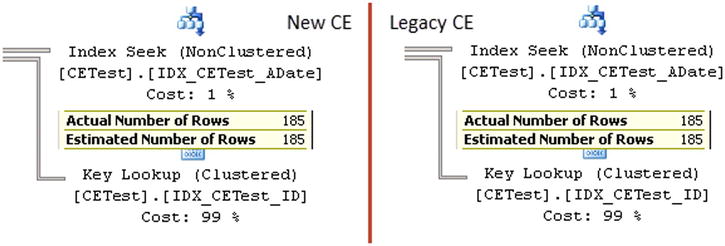
Figure 3-14. Up-to-date statistics: Cardinality estimations for value, which is a key in the histogram step
Now let’s run the query, which selects data for ADate = '2013-06-23', which is not present in the histogram as a key. Listing 3-14 illustrates the queries.
Listing 3-14. Up-to-date statistics: Selecting data for value, which is not a key in the histogram step
-- New Cardinality Estimator
select ID, ADate, Placeholder
from dbo.CETest with (index=IDX_CETest_ADate)
where ADate = '2013-06-23'

-- Legacy Cardinality Estimator
select ID, ADate, Placeholder
from dbo.CETest with (index=IDX_CETest_ADate)
where ADate = '2013-06-23'
option (querytraceon 9481)
Again, the results shown in Figure 3-15 are the same for both models. SQL Server uses the AVG_RANGE_ROWS column value from the 14th histogram step for the estimation.

Figure 3-15. Up-to-date statistics: Cardinality estimations for value, which is not a key in the histogram step
Finally, let’s run a parameterized query, as shown in Listing 3-15, using a local variable as the predicate. In this case, SQL Server uses average selectivity in the index and estimates the number of rows by multiplying the density of the key by the total number of rows in the index: 0.002739726 * 65536 = 179.551. Both models produce the same result, as shown in Figure 3-16.
Listing 3-15. Up-to-date statistics: Selecting data for unknown value
declare
        @D date = '2013-06-25'

-- New Cardinality Estimator
select ID, ADate, Placeholder
from dbo.CETest with (index=IDX_CETest_ADate)
where ADate = @D

-- Legacy Cardinality Estimator
select ID, ADate, Placeholder
from dbo.CETest with (index=IDX_CETest_ADate)
where ADate = @D
option (que2rytraceon 9481);

Figure 3-16. Up-to-date statistics: Cardinality estimations for an unknown value
As you can see, when the statistics are up to date, both models provide the same results.
Comparing Cardinality Estimators: Outdated Statistics
Unfortunately, in systems with non-static data, data modifications always outdate the statistics. Let’s look at how this affects cardinality estimations in both models and insert 6,554 new rows in the table, which is 10 percent of total number of rows. This number is below the statistics update threshold; therefore, SQL Server does not update the statistics. Listing 3-16 shows the code for achieving this.
Listing 3-16. Comparing Cardinality Estimators: Adding new rows
;with N1(C) as (select 0 union all select 0) -- 2 rows
,N2(C) as (select 0 from N1 as T1 cross join N1 as T2) -- 4 rows
,N3(C) as (select 0 from N2 as T1 cross join N2 as T2) -- 16 rows
,N4(C) as (select 0 from N3 as T1 cross join N3 as T2) -- 256 rows
,N5(C) as (select 0 from N4 as T1 cross join N4 as T2) -- 65,536 rows
,IDs(ID) as (select row_number() over (order by (select NULL)) from N5)
        insert into dbo.CETest(ID,ADate)
                select ID + 65536,dateadd(day,abs(checksum(newid())) % 365,'2013-06-01')
                from IDs
                where ID <= 6554;
Now let’s repeat our tests by running the queries from Listings 3-13, 3-14, and 3-15. Figure 3-17 illustrates the cardinality estimation for queries from Listing 3-13, where the value is present as a key in the histogram step. As you can see, both models estimated 203.498 rows, which is 10 percent more than previously. SQL Server compares the number of rows in the table with the original Rows value in the statistics and adjusted the value from the EQ_ROWS column in the 14th histogram step accordingly.
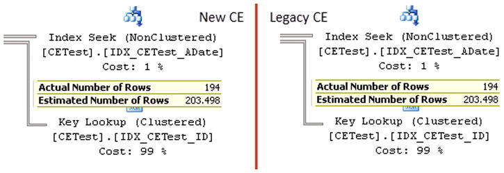
Figure 3-17. Outdated statistics: Cardinality estimations for the value, which is a key in the histogram step
Figure 3-18 shows the cardinality estimations for the queries from Listing 3-14 when the value is not a key in the histogram step. You can see the difference here. The new model takes the 10 percent difference in the row count into consideration, similar to the previous example. The legacy model, on the other hand, still uses the AVG_RANGE_ROWS value from the histogram step, even though the number of rows in the table does not match the number of rows kept in the statistics.
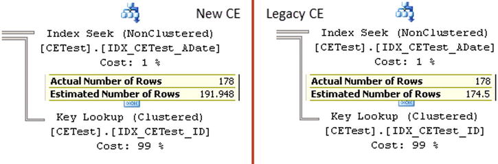
Figure 3-18. Outdated statistics: Cardinality estimations for the value, which is not a key in the histogram step
The same thing happens with the parameterized queries from Listing 3-15. The new model adjusts the estimation based on the row count differences, while the legacy model ignores them. Figure 3-19 illustrates these estimations.
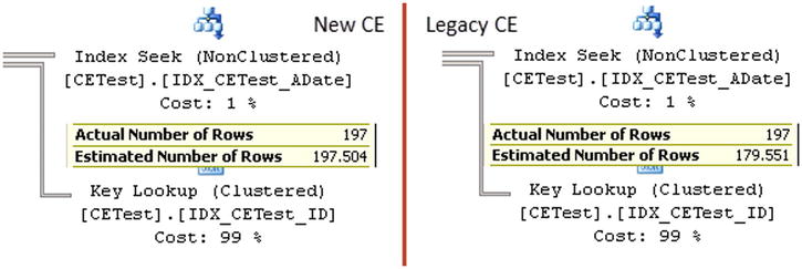
Figure 3-19. Outdated statistics: Cardinality estimations for an unknown value
Both approaches have their pros and cons. The new model produces better results when new data has been evenly distributed in the index. This is exactly what happened in our case when ADate values were randomly generated. Alternatively, the legacy model works better in the case of uneven distribution of new values when the distribution of old values did not change. You can think about indexes with ever-increasing key values as an example.
Comparing Cardinality Estimators: Indexes with Ever-Increasing Key Values
The next test compares behavior of cardinality estimators when the value is outside of the histogram range. This often happens in cases of indexes with ever-increasing key values, such as on the identity or sequence columns. Right now, we have such a situation with the IDX_CETest_ID index. Index statistics were not updated after we inserted new rows as shown in Figure 3-20.
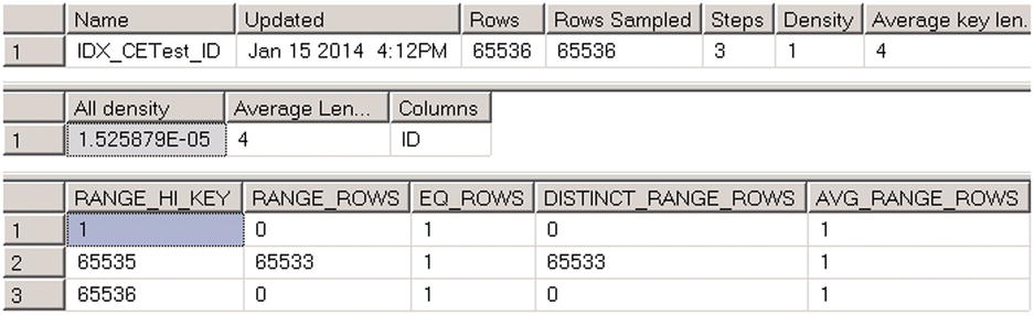
Figure 3-20. Indexes with ever-increasing keys: Histogram
Listing 3-17 shows the queries that select data for parameters, which are not present in the histogram. Figure 3-21 shows the cardinality estimations.
Listing 3-17. Indexes with ever-increasing key values: Test queries
-- New Cardinality Estimator
select top 10 ID, ADate
from dbo.CETest
where ID between 66000 and 67000
order by PlaceHolder;

-- Legacy Cardinality Estimator
select top 10 ID, ADate
from dbo.CETest
where ID between 66000 and 67000
order by PlaceHolder
option (querytraceon 9481);

Figure 3-21. Cardinality estimations for indexes with ever-increasing keys
As you can see, the legacy model estimated just the single row while the new model performed the estimation based on the average data distribution in the index. The new model provides better results and lets you avoid frequent manual statistics updates for indexes with ever-increasing key values.
Comparing Cardinality Estimators: Joins
Let’s look at how both models handle joins and create another table, as shown in Listing 3-18. The table has a single ID column populated with data from the CETest table and references it with a foreign key constraint.
Listing 3-18. Cardinality estimators and joins: Creating another table
create table dbo.CETestRef
(
        ID int not null,

        constraint FK_CTTestRef_CTTest
        foreign key(ID)
        references dbo.CETest(ID)
);

-- 72,089 rows
insert into dbo.CETestRef(ID)
        select ID from dbo.CETest;

create unique clustered index IDX_CETestRef_ID
on dbo.CETestRef(ID);
![]() Note We will discuss foreign key constraints in greater depth in Chapter 7, “Constraints.”
Note We will discuss foreign key constraints in greater depth in Chapter 7, “Constraints.”
As a first step, let’s run the query with a join, as shown in Listing 3-19. This query returns data from the CETestRef table only. A foreign-key constraint guarantees that every row in the CETestRef table has a corresponding row in the CETest table; therefore, SQL Server can eliminate the join from the execution plan.
Listing 3-19. Cardinality estimators and joins: Test query 1
select d.ID
from dbo.CETestRef d join dbo.CETest m on
        d.ID = m.ID
![]() Note We will discuss join elimination in greater depth in Chapter 9, “Views.”
Note We will discuss join elimination in greater depth in Chapter 9, “Views.”
Figure 3-22 shows the cardinality estimations for the query. As you can see, both models work the same, correctly estimating the number of rows.
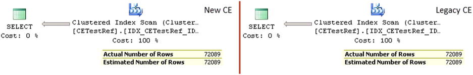
Figure 3-22. Cardinality estimations with join elimination
Let’s change our query and add a column from the referenced table to the result set. The code for doing this is shown in Listing 3-20.
Listing 3-20. Cardinality estimators and joins: Test query 2
select d.ID, m.ID
from dbo.CETestRef d join dbo.CETest m on
        d.ID = m.ID
Even though a foreign-key constraint guarantees that the number of rows in the result set will match the number of rows in the CETestRef table, the legacy cardinality estimator does not take it into consideration, and therefore underestimates the number of rows. The new cardinality estimator does a better job, providing the correct result. Figure 3-23 illustrates the latter.
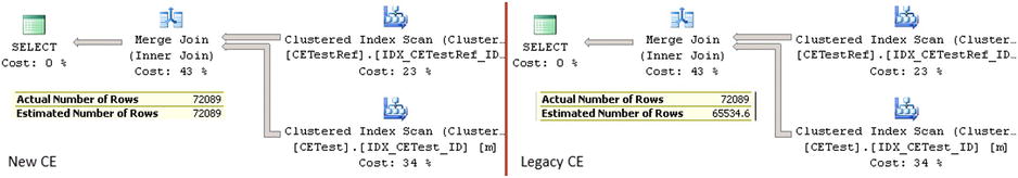
Figure 3-23. Cardinality estimations with join
It is worth mentioning that the new model does not always provide a 100 percent correct estimation when joins are involved. Nevertheless, the results are generally better than with the legacy model.
Comparing Cardinality Estimators: Multiple Predicates
The new cardinality estimation model removes the Independence assumption, and it expects some level of correlation between entities attributes. It performs estimations differently when queries have multiple predicates that involve multiple columns in the table. Listing 3-21 shows an example of such a query. Figure 3-24 shows the cardinality estimations for both models.
Listing 3-21. Query with multiple predicates
-- New Cardinality Estimator
select ID, ADate
from dbo.CETest
where
        ID between 20000 and 30000 and
        ADate between '2014-01-01' and '2014-02-01';

-- Legacy Cardinality Estimator
select ID, ADate
from dbo.CETest
where
        ID between 20000 and 30000 and
        ADate between '2014-01-01' and '2014-02-01';
option (querytraceon 9481)
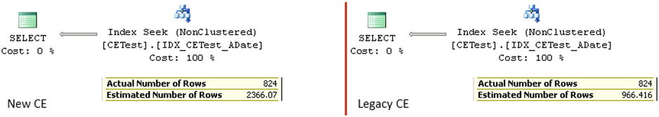
Figure 3-24. Cardinality estimations with multiple predicates
The legacy cardinality estimator assumes the independence of predicates and uses the following formula:
(Selectivity of first predicate * Selectivity of second predicate) * (Total number of rows in table) = (Estimated number of rows for first predicate * Estimated number of rows for second predicate) / (Total number of rows in the table).
The new cardinality estimator expects some correlation between predicates, and it uses another approach called an exponential backoff algorithm, which is as follows:
(Selectivity of most selective predicate) * SQRT(Selectivity of next most selective predicate) * (Total number of rows in table).
This change fits entirely into “It depends” category. The legacy cardinality estimator works better when there is no correlation between attributes/predicates, as shown in our example. The new cardinality estimator provides better results in cases of correlation. We will look at such an example in the “Filtered Statistics” section of the next chapter.
Summary
Correct cardinality estimation is one of the most important factors that allows the Query Optimizer to generate efficient execution plans. Cardinality estimation affects the choice of indexes, join strategies, and other parameters.
SQL Server uses statistics to perform cardinality estimations. The vital part of statistics is the histogram, which stores information about data distribution in the leftmost statistics column. Every step in the histogram contains a sample statistics column value and information about what happens in the interval defined by the step, such as how many rows are in the interval, how many unique key values are there, and so on.
SQL Server creates statistics for every index defined in the system. In addition, you can create column-level statistics on individual or multiple columns in the table. This can help SQL Server generate more efficient execution plans. In some cases, SQL Server creates column-level statistics automatically—if the database has the Auto Create Statistics database option enabled.
Statistics has a few limitations. There are at most 200 steps (key value intervals) stored in the histogram. As a result, the histogram’s steps cover larger key value intervals as the table grows. This leads to larger approximations within the interval and less accurate cardinality estimations on tables with millions or billions of rows.
Moreover, the histogram stores the information about data distribution for the leftmost statistics column only. There is no information about other columns in the statistics, aside from multi-column density.
SQL Server tracks the number of changes in statistics columns in the table. By default, SQL Server outdates and updates statistics after that number exceeds about 20 percent of the total number of the rows in the table. As a result, statistics are rarely updated automatically on large tables. You need to consider updating statistics on large tables manually based on some schedule. You should also update statistics on ever-increasing or ever-decreasing indexes more often because SQL Server tends to underestimate the number of rows when the parameters are outside of the histogram, unless you are using the new cardinality estimation model introduced in SQL Server 2014.
The new cardinality estimation model is enabled in SQL Server 2014 for databases with a compatibility level of 120. This model addresses a few common issues, such as estimations for ever-increasing indexes when statistics is not up-to-date; however, it may introduce plan regressions in some cases. You should carefully test existing systems before enabling the new cardinality estimation model after upgrading SQL Server.