![]()
Things do not always work as expected. System performance can degrade over time when the amount of data and load increases, or sometimes a server can become unresponsive and stop accepting any connections at all. In either case, you need to find and fix such problems quickly while working under pressure and stress.
In this chapter, we will talk about the SQL Server execution model and discuss system troubleshooting based on Wait Statistics Analysis. I will show you how to detect common issues frequently encountered in systems.
Looking at the Big Picture
Even though this chapter focuses on the troubleshooting of database-related issues, you need to remember that databases and SQL Server never live in a vacuum. There are always the customers who use client applications. Those applications work with single or multiple databases from one or more instances of SQL Server. SQL Server, in turn, runs on physical or virtual hardware, with data stored on disks often shared with other customers and database systems. Finally, all system components use the network for communication and network-based storage access.
From the customers’ standpoint, most problems present themselves as general performance issues. Client applications feel slow and unresponsive, queries time-out and, in some cases, applications cannot even connect to the database. Nevertheless, the root-cause of the problem could be anywhere. Hardware could be malfunctioning or incorrectly configured; the database might have inefficient schema, indexing, or code, SQL Server could be overloaded, or client applications could have bugs or design issues.
![]() Important You should always look at all of the components of a system during troubleshooting and identify the root-cause of the problem.
Important You should always look at all of the components of a system during troubleshooting and identify the root-cause of the problem.
The performance of a system depends on its slowest component. For example, if SQL Server uses SAN storage, you should look at the performance of both the storage subsystem and the network. If network throughput is not sufficient to transmit data, improving SAN performance wouldn’t help much. You could achieve better results by optimizing network throughput or by reducing the amount of network traffic with extra indexes or database schema changes.
Another example is client-side data processing when a large amount of data needs to be transmitted to client applications. While you can improve application performance by upgrading a network, you could obtain much better results by moving the data processing to SQL and/or Application Servers, thereby reducing the amount of data travelling over the wire.
In this chapter, we will focus on troubleshooting the database portion of the system. However, I would still like to mention the various components and configuration settings that you should analyze during the initial stage of performance troubleshooting. Do not consider this list to be a comprehensive guide on hardware and software configuration. Be sure to do further research using Microsoft TechNet documentation, White Papers, and other resources, especially when you need to deploy, configure, or troubleshoot complex infrastructures.
Hardware and Network
As a first step in troubleshooting, it is beneficial to look at the SQL Server hardware and network configuration. There are several aspects of this involved. First, it makes sense to analyze if the server is powerful enough to handle the load. Obviously, this is a very subjective question, which often cannot be answered based solely on the server specifications. However, in some cases, you will see that the hardware is clearly underpowered.
One example when this happens is with systems developed by Independent Software Vendors (ISV) and deployed in an Enterprise environment. Such deployments usually happen in stages. Decision makers evaluate system functionality under a light load during the trial/pilot stage. It is entirely possible that the database has been placed into second-grade hardware or an under-provisioned virtual machine during trials and stayed there even after full deployment.
SQL Server is a very I/O intensive application, and a slow or misconfigured I/O subsystem often becomes a performance bottleneck. One very important setting that is often overlooked is partition alignment. Old versions of Windows created partitions right after 63 hidden sectors on a disk, which striped the disk allocation unit across multiple stripe units in RAID arrays. With such configurations, a single I/O request to a disk controller leads to multiple I/O operations to access data from the different RAID stripes.
Fortunately, partitions created in Windows Server 2008 and above are aligned by default. However, Windows does not re-align existing partitions created in older versions of Windows when you upgrade operating systems or attach disks to servers. It is possible to achieve a 20-40 percent I/O performance improvement by fixing an incorrect partition alignment without making any other changes to the system.
Windows allocation unit size also comes into play. Most SQL Server instances would benefit from 64KB units, however you should take the RAID stripe size into account. Use the RAID stripe size recommended by the manufacturer; however, make sure that the Windows allocation unit resides on the single RAID stripe. For example, a 1MB RAID stripe size works fine with 64KB windows allocation units hosting 16 allocation units per stripe when disk partitions are aligned.
![]() Tip You can read more about partition alignments at: http://technet.microsoft.com/en-us/library/dd758814.aspx.
Tip You can read more about partition alignments at: http://technet.microsoft.com/en-us/library/dd758814.aspx.
Finally, you need to analyze network throughput. Network performance depends on the slowest link in the topology. This is especially important in cases of network-based storage when every physical I/O operation utilizes the network. For example, if one of the network switches in the path between SQL Server and a SAN has 2-gigabit uplink, the network throughput would be limited to 2 gigabits, even when all other network components in the topology are faster than that. Moreover, always remember to factor in the distance information travels over a network. Accessing remote data adds extra latency and slows down communications.
Operating System Configuration
You should look at the operating system configuration in the next step. It is especially important in the case of a 32-bit OS where the amount of user memory available to processes is limited. It is crucial that you check that SQL Server can use extended memory and that the “Use AWE Memory” setting is enabled.
![]() Note The 32-bit version of SQL Server can use extended memory for the buffer pool only. This limits the amount of memory that can be utilized by other components, such as plan cache and lock manager. It is always beneficial to upgrade to a 64-bit version of SQL Server if possible.
Note The 32-bit version of SQL Server can use extended memory for the buffer pool only. This limits the amount of memory that can be utilized by other components, such as plan cache and lock manager. It is always beneficial to upgrade to a 64-bit version of SQL Server if possible.
You should check what software is installed and what processes are running on the server. Non-essential processes use memory and contribute to server CPU load. Think about anti-virus software as an example. It is better to protect the server from viruses by restricting user access and revoking administrator permissions, rather than to have anti-virus software constantly running on the server. If company policy requires that you have anti-virus up and running, make sure that the system and user databases are excluded from the scan.
Using development and troubleshooting tools locally on the server is another commonly encountered mistake. Developers and database administrators often run Management Studio, SQL Profiler, and other tools on a server during deployment and troubleshooting. Those tools reduce the amount of memory available to SQL Server and contribute to unnecessary load. It is always better to access SQL Server remotely whenever possible.
Also check if SQL Server is virtualized. Virtualization helps reduce IT costs, improves the availability of the system, and simplifies management. However, virtualization adds another layer of complexity during performance troubleshooting. Work with system administrators, or use third-party tools, to make sure that the host is not overloaded, even when performance metrics in a guest virtual machine appear normal.
Another common problem related to virtualization is resource over-allocation. As an example, it is possible to configure a host in such a way that the total amount of memory allocated for all guest virtual machines exceeds the amount of physical memory installed on the host. That configuration leads to artificial memory pressure and introduces performance issues for a virtualized SQL Server. Again, you should work with system administrators to address such situations.
SQL Server Configuration
It is typical to have multiple databases hosted on a SQL Server instance. Database consolidation helps lower IT costs by reducing the number of servers that you must license and maintain. All those databases, however, use the same pool of SQL Server resources, contribute to its load, and affect each other. Heavy SQL Server workload from one system can negatively impact the performance of other systems.
You can analyze such conditions by examining resource-intensive and frequently executed queries on the server scope. If you detect a large number of such queries coming from different databases, you may consider optimizing all of them or to separate the databases among different servers. We will discuss how to detect such queries later in this chapter.
![]() Tip Starting with SQL Server 2008, you can throttle CPU activity and query execution memory for sessions using Resource Governor. In addition, SQL Server 2014 allows you to throttle I/O activity. Resource Governor is available in the Enterprise Edition only, and it does not allow you to throttle buffer pool usage.
Tip Starting with SQL Server 2008, you can throttle CPU activity and query execution memory for sessions using Resource Governor. In addition, SQL Server 2014 allows you to throttle I/O activity. Resource Governor is available in the Enterprise Edition only, and it does not allow you to throttle buffer pool usage.
You can read more about Resource Governor at: http://msdn.microsoft.com/en-us/library/bb933866.aspx.
You should also check if multiple SQL Server instances are running on the same server and how they affect the performance of each other. This condition is a bit trickier to detect and requires you to analyze various performance counters and DMOs from multiple instances. One of the most common problems in this situation happens when multiple SQL Server instances compete for memory, introducing memory pressure on each other. It might be beneficial to set and fine-tune the minimum and maximum memory settings for each instance based on requirements and load.
It is also worth noting that various Microsoft and third-party products often install separate SQL Server instances without your knowledge. Always check to see if this is the case on non-dedicated servers.
![]() Tip In SQL Server versions prior to 2012, Minimum and Maximum Server Memory settings controlled only the size of the buffer pool. You should reserve additional memory for other SQL Server components in versions prior to SQL Server 2012.
Tip In SQL Server versions prior to 2012, Minimum and Maximum Server Memory settings controlled only the size of the buffer pool. You should reserve additional memory for other SQL Server components in versions prior to SQL Server 2012.
Finally, check the tempdb configuration and make sure that it is optimal, as we have already discussed in Chapter 12, “Temporary Tables.”
DATABASE CONSOLIDATION
It is impossible to avoid discussion about the database consolidation process when we talk about SQL Server installations hosting multiple databases. Even though it is not directly related to the topic of the chapter, I would like to review several aspects of the database consolidation process here.
There is no universal consolidation strategy that can be used with every project. You should analyze the amount of data, load, hardware configuration, and business and security requirements when making this decision. However, as a general rule, you should avoid consolidating OLTP and Data Warehouse/Reporting databases on the same server when they are working under a heavy load. Data Warehouse queries usually process large amounts of data, which leads to heavy I/O activity and flushes the content of the buffer pool. Taken together, this negatively affects the performance of other systems.
Listing 27-1 shows you how to get information about buffer pool usage on a per-database basis. Moreover, the sys.dm_io_virtual_file_stats function can provide you with statistics about the I/O activity for each database file. We will discuss this function in greater detail later in this chapter.
Listing 27-1. Buffer pool usage on per-database basis
Select
database_id as [DB ID]
,db_name(database_id) as [DB Name]
,convert(decimal(11,3),count(*) * 8 / 1024.0) as
[Buffer Pool Size (MB)]
from sys.dm_os_buffer_descriptors with (nolock)
group by database_id
order by [Buffer Pool Size (MB)] desc
option (recompile);
You should also analyze the security requirements when consolidating databases. Some security features, such as Audit, work on the server scope and add performance overhead for all of the databases on the server. Transparent Data Encryption (TDE) is another example. Even though it is a database-level feature, SQL Server encrypts tempdb when either of the databases has TDE enabled, which also introduces performance overhead for other systems.
As a general rule, you should avoid consolidating databases with different security requirements on the same instance of SQL Server. Using multiple instances of SQL Server is a better choice, even when such instances run on the same server.
Database Options
Every database should have the Auto Shrink option disabled. As we have already discussed, the Auto Shrink periodically triggers the database shrink process, which introduces unnecessary I/O load and heavy index fragmentation. Moreover, this operation is practically useless because further data modifications and index maintenance make database files grow yet again.
The Auto Close option forces SQL Server to remove any database-related objects from memory when the database does not have any connected users. As you can guess, it leads to extra physical I/O and query compilations as users reconnect to the database afterwards. With the rare exception of very infrequently accessed databases, the Auto Close setting should be disabled.
It is better to have multiple data files in filegroups with volatile data. This helps avoid allocation map contention, similar to what happens in the case of tempdb. We will discuss the symptoms of such contention later in this chapter.
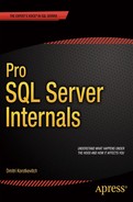
From a high level, the architecture of SQL Server includes five different components, as shown in Figure 27-1.
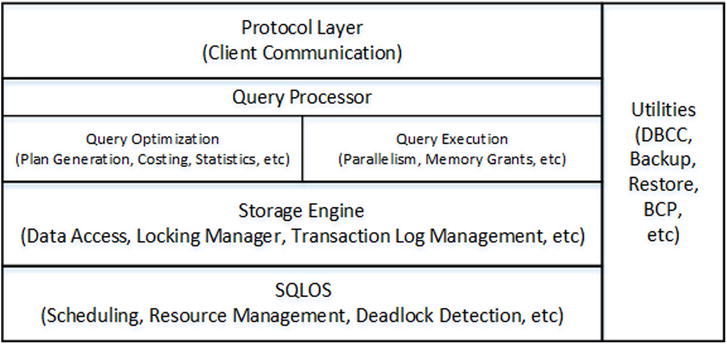
Figure 27-1. High-Level SQL Server Architecture
The Protocol layerhandles communications between SQL Server and the client applications. The data is transmitted in an internal format called Tabular Data Stream (TDS) using one of the standard network communication protocols, such as TCP/IP or Name Pipes. Another communication protocol, called Shared Memory, can be used when both SQL Server and client applications run locally on the same server. The shared memory protocol does not utilize the network and is more efficient than the others.
![]() Tip Different editions of SQL Server have different protocols enabled after installation. For example, the SQL Server Express Edition has all network protocols disabled by default, and it would not be able to serve network requests until you enable them. You can enable and disable protocols in the SQL Server Configuration Manager Utility.
Tip Different editions of SQL Server have different protocols enabled after installation. For example, the SQL Server Express Edition has all network protocols disabled by default, and it would not be able to serve network requests until you enable them. You can enable and disable protocols in the SQL Server Configuration Manager Utility.
The Query Processor layer is responsible for query optimization and execution. We have already discussed various aspects of its behavior in previous chapters.
The Storage Engine consists of components related to data access and data management in SQL Server. It works with the data on disk, handles transactions and concurrency, manages the transaction log, and performs several other functions.
SQL Server includes a set of Utilities, which are responsible for backup and restore operations, bulk loading of data, full-text index management, and several other actions.
Finally, the vital component of SQL Server is the SQL Server Operating System (SQLOS). SQLOS is the layer between SQL Server and Windows, and it is responsible for scheduling and resource management, synchronization, exception handling, deadlock detection, CLR hosting, and more. For example, when any SQL Server component needs to allocate memory, it does not call the Windows API function directly, but rather it requests memory from SQLOS, which in turn uses the memory allocator component to fulfill the request.
![]() Note The Enteprise Edition of SQL Server 2014 includes another major component called, “In-Memory OLTP Engine.” We will discuss this component in more detail in Part 7, “In-Memory OLTP Engine (Hekaton).”
Note The Enteprise Edition of SQL Server 2014 includes another major component called, “In-Memory OLTP Engine.” We will discuss this component in more detail in Part 7, “In-Memory OLTP Engine (Hekaton).”
SQLOS was initially introduced in SQL Server 7.0 to improve the efficiency of scheduling in SQL Server and to minimize context and kernel mode switching. The major difference between Windows and SQLOS is the scheduling model. Windows is a general-purpose operating system that uses preemptive scheduling. It controls what processes are currently running, suspending, and resuming them as needed. Alternatively, with the exception of CLR code, SQLOS uses cooperative scheduling when processes yield voluntarily on a regular basis.
SQLOS creates a set of schedulers when it starts. The number of schedulers is equal to the number of logical CPUs in the system. For example, if a server has two quad-core CPUs with Hyper-Threading enabled, SQL Server creates 16 schedulers. Each scheduler can be in either an ONLINE or OFFLINE stage based on the process affinity settings and core-based licensing model.
Even though the number of schedulers matches the number of CPUs in the system, there is no strict one-to-one relationship between them unless the process affinity settings are enabled. In some cases, and under heavy load, it is possible to have more than one scheduler running on the same CPU. Alternatively, when process affinity is set, schedulers are bound to CPUs in a strict one-to-one relationship.
Each scheduler is responsible for managing working threads called workers. The maximum number of workers in a system is specified by the Max Worker Thread configuration option. Each time there is a task to execute; it is assigned to a worker in an idle state. When there are no idle workers, the scheduler creates the new one. It also destroys idle workers after 15 minutes of inactivity or in case of memory pressure.
Workers do not move between schedulers. Moreover, a task is never moved between workers. SQLOS, however, can create child tasks and assign them to different workers, for example in the case of parallel execution plans.
Each task can be in one of six different states:
- Pending: Task is waiting for an available worker
- Done: Task is completed
- Running: Task is currently executing on the scheduler
- Runnable: Task is waiting for the scheduler to be executed
- Suspended: Task is waiting for external event or resource
- Spinloop: Task is processing a spinlock
![]() Note Spinlock is an internal lightweight synchronization mechanism that protects access to data structures. Coverage of spinlock is beyond the scope of this book. You can obtain more information about the troubleshooting of spinlock contention-related issues at: http://www.microsoft.com/en-us/download/details.aspx?id=26666.
Note Spinlock is an internal lightweight synchronization mechanism that protects access to data structures. Coverage of spinlock is beyond the scope of this book. You can obtain more information about the troubleshooting of spinlock contention-related issues at: http://www.microsoft.com/en-us/download/details.aspx?id=26666.
Each scheduler has at most one task in running state. In addition, it has two different queues—one for runnable tasks and one for suspended tasks. When the running task needs some resources—a data page from a disk, for example—it submits an I/O request and changes the state to suspended. It stays in the suspended queue until the request is fulfilled and the page is read. After that, the task is moved to the runnable queue when it is ready to resume execution.
![]() Note A grocery store is, perhaps, the closest real-life analogy to the SQL Server Execution Model. Think of cashiers as representing schedulers and customers in checkout lines are similar to tasks in the runnable queue. A customer who is currently checking out is similar to a task in the running state.
Note A grocery store is, perhaps, the closest real-life analogy to the SQL Server Execution Model. Think of cashiers as representing schedulers and customers in checkout lines are similar to tasks in the runnable queue. A customer who is currently checking out is similar to a task in the running state.
If item is missing a UPC code, a cashier sends a store worker to do a price check. The cashier suspends the checkout process for the current customer, asking her or him to step aside (to the suspended queue). When the worker comes back with the price information, the customer who had stepped aside moves to the end of the checkout line (end of the runnable queue).
It is worth mentioning that the SQL Server process is much more efficient as compared to real-life, when others wait patiently in-line during a price check. However, a customer who is forced to move to the end of the runnable queue would probably disagree with such a conclusion.
Figure 27-2 illustrates the typical task life cycle of the SQL Server Execution Model. The total task execution time can be calculated as a summary of the time task spent in the running state (when it ran on the scheduler), runnable state (when it waited for an available scheduler), and in suspended state (when it waited for a resource or external event).
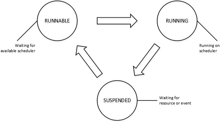
Figure 27-2. Task life cycle
SQL Server tracks the cumulative time tasks spend in suspended state for different types of waits and exposes this through the sys.dm_os_wait_tasks view. This information is collected as of the time of the last SQL Server restart or since it was cleared with the DBCC SQLPERF('sys.dm_os_wait_stats', CLEAR) command.
Listing 27-2 shows how to find top wait types in the system, which are the wait types for which workers spent the most time waiting. It is filtering out some nonessential wait types mainly related to internal SQL Server processes. Even though it is beneficial to analyze some of them during advanced performance tuning, you rarely focus on them during the initial stage of system troubleshooting.
Listing 27-2. Detecting top wait types in the system
;with Waits
as
(
        select
                wait_type, wait_time_ms, waiting_tasks_count,
                100. * wait_time_ms / SUM(wait_time_ms) over() as Pct,
                row_number() over(order by wait_time_ms desc) AS RowNum
        from sys.dm_os_wait_stats with (nolock)
        where
                wait_type not in /* Filtering out non-essential system waits */
        (N'CLR_SEMAPHORE',N'LAZYWRITER_SLEEP',N'RESOURCE_QUEUE'
        ,N'SLEEP_TASK',N'SLEEP_SYSTEMTASK',N'SQLTRACE_BUFFER_FLUSH'
        ,N'WAITFOR',N'LOGMGR_QUEUE',N'CHECKPOINT_QUEUE'
        ,N'REQUEST_FOR_DEADLOCK_SEARCH',N'XE_TIMER_EVENT'
        ,N'BROKER_TO_FLUSH',N'BROKER_TASK_STOP',N'CLR_MANUAL_EVENT'
        ,N'CLR_AUTO_EVENT',N'DISPATCHER_QUEUE_SEMAPHORE'
        ,N'FT_IFTS_SCHEDULER_IDLE_WAIT',N'XE_DISPATCHER_WAIT'
        ,N'XE_DISPATCHER_JOIN',N'SQLTRACE_INCREMENTAL_FLUSH_SLEEP'
        ,N'ONDEMAND_TASK_QUEUE',N'BROKER_EVENTHANDLER',N'SLEEP_BPOOL_FLUSH'
        ,N'SLEEP_DBSTARTUP',N'DIRTY_PAGE_POLL',N'BROKER_RECEIVE_WAITFOR'
        ,N'HADR_FILESTREAM_IOMGR_IOCOMPLETION', N'WAIT_XTP_CKPT_CLOSE'
        ,N'SP_SERVER_DIAGNOSTICS_SLEEP',N'BROKER_TRANSMITTER'
        ,N'QDS_PERSIST_TASK_MAIN_LOOP_SLEEP','MSQL_XP'
        ,N'QDS_CLEANUP_STALE_QUERIES_TASK_MAIN_LOOP_SLEEP'
        ,N'WAIT_XTP_HOST_WAIT', N'WAIT_XTP_OFFLINE_CKPT_NEW_LOG')
)
select
        w1.wait_type as [Wait Type]
        ,w1.waiting_tasks_count as [Wait Count]
        ,convert(decimal(12,3), w1.wait_time_ms / 1000.0) as [Wait Time]
        ,CONVERT(decimal(12,1), w1.wait_time_ms /
                                w1.waiting_tasks_count) as [Avg Wait Time]
        ,convert(decimal(6,3), w1.Pct) as [Percent]
        ,convert(decimal(6,3), sum(w2.Pct)) as [Running Percent]
from
        Waits w1 join Waits w2 on
                w2.RowNum <= w1.RowNum
group by
        w1.RowNum, w1.wait_type, w1.wait_time_ms, w1.waiting_tasks_count, w1.Pct
having
        sum(w2.Pct) - w1.pct < 95
option (recompile);
![]() Note Every new version of SQL Server introduces new wait types. You can see a list of wait types at: http://msdn.microsoft.com/en-us/library/ms179984.aspx. Make sure to select the appropriate version of SQL Server.
Note Every new version of SQL Server introduces new wait types. You can see a list of wait types at: http://msdn.microsoft.com/en-us/library/ms179984.aspx. Make sure to select the appropriate version of SQL Server.
Figure 27-3 illustrates the output of the script from one of the production servers at the beginning of the troubleshooting process. We will talk about wait types from output later in this chapter.
Figure 27-3. Output of the script on one of the production servers
There are other useful SQLOS related data management views:
- sys.dm_os_waiting_tasks returns the list of currently suspended tasks including wait type, waiting time, and the resource for which it is waiting. It also includes the id of the blocking session, if any.
- The sys.dm_exec_requests view provides the list of requests currently executing on SQL Server. This includes information about the session that submits the request; the current status of request; information about the current wait type if a task is suspended; SQL and plan handles; execution statistics, and several other attributes.
- The sys.dm_os_schedulers view returns information about schedulers, including their status, workers, and task information.
- The sys.dm_os_threads view provides information about workers.
- The sys.dm_os_tasks view provides information about tasks including their state and some execution statistics.
Wait Statistics Analysis and Troubleshooting
The process of analyzing top waits in the system is called Wait Statistics Analysis. This is one of the frequently used troubleshooting and performance tuning techniques in SQL Server. Figure 27-4 illustrates a typical Wait Statistics Analysis troubleshooting cycle.

Figure 27-4. Wait Statistics Analysis troubleshooting cycle
As a first step, you look at the wait statistics, which are detecting the top waits in the system. This narrows the area of concern for further analysis. After that, you confirm the problem using other tools, such as DMV, Windows Performance Monitor, SQL Traces and Extended Events, and detect the root-cause of the problem. When the root-cause is confirmed, you fix it and analyze the wait statistics again, choosing a new target for analysis and improvement.
This is a never-ending process. Waits always exist in systems, and there is always space for improvements. However, a generic 80/20 Pareto principle can be applied to almost any troubleshooting and optimization process. You achieve an 80 percent effect or improvement by spending 20 percent of your time. At some point, further optimization does not provide a sufficient return on investment and it is better to spend your time and resources elsewhere.
Even though wait statistics can help you detect problematic areas in a system, it is not always easy to find the root-cause of a problem. Different issues affect and often mask each other.
Figure 27-5 illustrates such a situation. Bad system performance due to a slow and unresponsive I/O subsystem often occurs due to missing indexes and non-optimized queries that overloaded it. Those queries require SQL Server to scan a large amount of data, which flushes the content of the buffer pool and contributes to CPU load. Moreover, missing indexes introduce locking and blocking in the system.
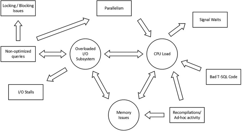
Figure 27-5. Everything is related
Ad-hoc queries and recompilations contribute to CPU load and increase plan cache size, which in turn leaves less memory for the buffer pool. It is also increases I/O subsystem load due to the extra physical I/O required.
Let’s look at different issues frequently encountered in systems and discuss how we can detect and troubleshoot them.
I/O Subsystem and Non-Optimized Queries
The most common root-cause of issues related to a slow and/or overloaded I/O subsystem is non-optimized queries, which require SQL Server to scan a large amount of data. When SQL Server does not have enough physical memory to cache all of the required data in the buffer pool, which is typically the case for large systems, physical I/O occurs and constantly replaces data in the buffer pool.
![]() Tip You can add or allocate more physical memory to the server that hosts SQL Server when an I/O subsystem is overloaded. Extra memory increases the size of the buffer pool and the amount of data SQL Server can cache. It reduces the physical I/O required to scan the data. While it did not fix the root-cause of the problem, it could work as an emergency Band-Aid technique and buy you some time. Remember that non-Enterprise editions of SQL Server have limitations in the amount of memory that they can utilize.
Tip You can add or allocate more physical memory to the server that hosts SQL Server when an I/O subsystem is overloaded. Extra memory increases the size of the buffer pool and the amount of data SQL Server can cache. It reduces the physical I/O required to scan the data. While it did not fix the root-cause of the problem, it could work as an emergency Band-Aid technique and buy you some time. Remember that non-Enterprise editions of SQL Server have limitations in the amount of memory that they can utilize.
Figure 27-6 illustrates the situation with non-optimized queries, and it shows the metrics and tools that can be used to diagnose and fix these problems.
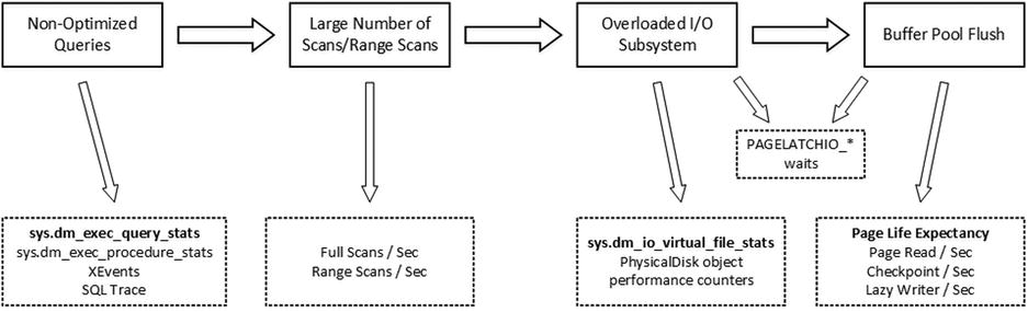
Figure 27-6. Non-optimized queries troubleshooting
PAGEIOLATCH_* wait types occur when SQL Server is waiting for an I/O subsystem to bring a data page from disk to the buffer pool. A large percentage of those waits indicate heavy physical I/O activity in the system. Other I/O wait types, such as IO_COMPLETION, ASYNC_IO_COMPLETION, BACKUPIO, WRITELOG, and LOGBUFFER relate to non-data pages I/O. Those wait types may occur for various reasons. IO_COMPLETION often indicates slow tempdb I/O performance during sort and hash operators. BACKUPIO is a sign of slow performance of a backup disk drive, and it often occurs with an ASYNC_IO_COMPLETION wait type. WRITELOG and LOGBUFFER waits are a sign of bad transaction log I/O throughput.
When all of those wait types are present together, it is easier to focus on reducing PAGEIOLATCH waits and data-related I/O. This will reduce the load on the I/O subsystem and, in turn, it can improve the performance of non-data–related I/O operations. Otherwise, when PAGEIOLATCH waits are not very significant, you need to look at I/O subsystem performance and configuration and correlate the data from the various metrics we are about to discuss.
![]() Tip One common case where you have non-data pages I/O related waits without PAGEIOLATCH waits present is when SQL Server has a slow I/O subsystem and enough memory to cache frequently accessed data.
Tip One common case where you have non-data pages I/O related waits without PAGEIOLATCH waits present is when SQL Server has a slow I/O subsystem and enough memory to cache frequently accessed data.
The sys.dm_io_virtual_file_stats function provides you with I/O statistics for data and log files including information about a number of I/O operations, the amount of data processed, and I/O stalls, which is the time that SQL Server waited for I/O operations to complete. This can help you detect most I/O intensive databases and data files, which is especially useful when a SQL Server instance hosts a large number of databases.
![]() Tip You can use the sys.dm_io_virtual_file_stats function to monitor I/O load on a per-database basis when you are working on database consolidation projects.
Tip You can use the sys.dm_io_virtual_file_stats function to monitor I/O load on a per-database basis when you are working on database consolidation projects.
Listing 27-3 shows you the query that obtains information about I/O statistics for all of the databases on a server. Figure 27-7 illustrates the partial output of the query from one of the production servers.
Listing 27-3. Using sys.dm_io_virtual_file_stats
select
        fs.database_id as [DB ID]
        ,fs.file_id as [File Id]
        ,mf.name as [File Name]
        ,mf.physical_name as [File Path]
        ,mf.type_desc as [Type]
        ,fs.sample_ms as [Time]
        ,fs.num_of_reads as [Reads]
        ,fs.num_of_bytes_read as [Read Bytes]
        ,fs.num_of_writes as [Writes]
        ,fs.num_of_bytes_written as [Written Bytes]
        ,fs.num_of_reads + fs.num_of_writes as [IO Count]
        ,convert(decimal(5,2),100.0 * fs.num_of_bytes_read /
                (fs.num_of_bytes_read + fs.num_of_bytes_written)) as [Read %]
        ,convert(decimal(5,2),100.0 * fs.num_of_bytes_written /
                (fs.num_of_bytes_read + fs.num_of_bytes_written)) as [Write %]
        ,fs.io_stall_read_ms as [Read Stall]
        ,fs.io_stall_write_ms as [Write Stall]
        ,case when fs.num_of_reads = 0
                then 0.000
                else convert(decimal(12,3),1.0 *
                        fs.io_stall_read_ms / fs.num_of_reads)
        end as [Avg Read Stall]
        ,case when fs.num_of_writes = 0
                then 0.000
                else convert(decimal(12,3),1.0 *
                        fs.io_stall_write_ms / fs.num_of_writes)
        end as [Avg Write Stall]
from
        sys.dm_io_virtual_file_stats(null,null) fs join
                sys.master_files mf with (nolock) on
                        fs.database_id = mf.database_id and
                        fs.file_id = mf.file_id
        join sys.databases d with (nolock) on
                d.database_id = fs.database_id
where
        fs.num_of_reads + fs.num_of_writes > 0
option (recompile)
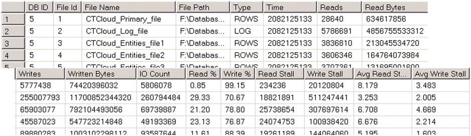
Figure 27-7. Sys_dm_io_virtual_file_stats output
Unfortunately, sys.dm_io_virtual_file_stats provides cumulative statistics as of the time of a SQL Server restart without any way to clear it. If you need to get a snapshot of the current load in the system, you should run this function several times and compare how the results changed between calls. Listing 27-4 shows the code that allows you to do that.
Listing 27-4. Using sys.dm_io_virtual_file_stats to obtain statistics about the current I/O load
create table #Snapshot
(
        database_id smallint not null,
        file_id smallint not null,
        num_of_reads bigint not null,
        num_of_bytes_read bigint not null,
        io_stall_read_ms bigint not null,
        num_of_writes bigint not null,
        num_of_bytes_written bigint not null,
        io_stall_write_ms bigint not null
);

insert into #Snapshot(database_id,file_id,num_of_reads,num_of_bytes_read
        ,io_stall_read_ms,num_of_writes,num_of_bytes_written
        ,io_stall_write_ms)
        select database_id,file_id,num_of_reads,num_of_bytes_read
                ,io_stall_read_ms,num_of_writes,num_of_bytes_written
                ,io_stall_write_ms
        from sys.dm_io_virtual_file_stats(NULL,NULL)
option (recompile);

-- Set test interval (1 hour)
waitfor delay '00:01:00.000';

;with Stats(db_id, file_id, Reads, ReadBytes, Writes
        ,WrittenBytes, ReadStall, WriteStall)
as
(
        select
                s.database_id, s.file_id
                ,fs.num_of_reads - s.num_of_reads
                ,fs.num_of_bytes_read - s.num_of_bytes_read
                ,fs.num_of_writes - s.num_of_writes
                ,fs.num_of_bytes_written - s.num_of_bytes_written
                ,fs.io_stall_read_ms - s.io_stall_read_ms
                ,fs.io_stall_write_ms - s.io_stall_write_ms
        from
                #Snapshot s cross apply
                        sys.dm_io_virtual_file_stats(s.database_id, s.file_id) fs
)
select
        s.db_id as [DB ID], d.name as [Database]
        ,mf.name as [File Name], mf.physical_name as [File Path]
        ,mf.type_desc as [Type], s.Reads
        ,convert(decimal(12,3), s.ReadBytes / 1048576.) as [Read MB]
        ,convert(decimal(12,3), s.WrittenBytes / 1048576.) as [Written MB]
        ,s.Writes, s.Reads + s.Writes as [IO Count]
        ,convert(decimal(5,2),100.0 * s.ReadBytes /
                        (s.ReadBytes + s.WrittenBytes)) as [Read %]
        ,convert(decimal(5,2),100.0 * s.WrittenBytes /
                        (s.ReadBytes + s.WrittenBytes)) as [Write %]
        ,s.ReadStall as [Read Stall]
        ,s.WriteStall as [Write Stall]
        ,case when s.Reads = 0
                then 0.000
                else convert(decimal(12,3),1.0 * s.ReadStall / s.Reads)
        end as [Avg Read Stall]
        ,case when s.Writes = 0
                then 0.000
                else convert(decimal(12,3),1.0 * s.WriteStall / s.Writes)
        end as [Avg Write Stall]
from
        Stats s join sys.master_files mf with (nolock) on
                s.db_id = mf.database_id and
                s.file_id = mf.file_id
        join sys.databases d with (nolock) on
                s.db_id = d.database_id
where
        s.Reads + s.Writes > 0
order by
        s.db_id, s.file_id
option (recompile)
You can analyze various system performance counters from the PhysicalDisk object to obtain information about current I/O activity, such as the number of requests and the amount of data being read and written. Those counters, however, are the most useful when compared against the baseline, which we will discuss later in this chapter.
Performance counters from the Buffer Manager Object provide various metrics related to the buffer pool and data page I/O. One of the most useful counters is Page Life Expectancy, which indicates the average time a data page stays in the buffer pool. Historically, Microsoft suggested that values above 300 seconds are acceptable and good enough, however this is hardly the case with modern servers that use large amounts of memory. One approach to defining the lowest-acceptable value for the counter is by multiplying 300 seconds for every 4GB of buffer pool memory. For example, a server that uses 56GB of memory for the buffer pool should have a Page Life Expectancy greater than 4,200 seconds (56/4*300). However, as with other counters, it is better to compare the current value against a baseline, rather than relying on a statically defined threshold.
Page Read/Secand Page Write/Sec counters show the number of physical data pages that were read and written respectively. Checkpoint Pages/Sec and Lazy Writer/Sec indicate the activity of the checkpoint and lazy writer processes that save dirty pages to disks. High numbers in those counters and a low value for Page Life Expectancy could be a sign of memory pressure. However, a high number of checkpoints could transpire due to a large number of transactions in the system, and you should include the Transactions/Sec counter in the analysis.
The Buffer Cache Hit Ratioindicates the percentage of pages that are found in the buffer pool without the requirement of performing a physical read operation. A low value in this counter indicates a constant buffer pool flush and is a sign of a large amount of physical I/O. However, a high value in the counter is meaningless. Read-ahead reads often bring data pages to memory, increasing the Buffer Cache Hit Ratio value and masking the problem. In the end, Page Life Expectancy is a more reliable counter for this analysis.
![]() Note You can read more about performance counters from the Buffer Manager Object at: http://technet.microsoft.com/en-us/library/ms189628.aspx.
Note You can read more about performance counters from the Buffer Manager Object at: http://technet.microsoft.com/en-us/library/ms189628.aspx.
Full Scans/Sec and Range Scan/Sec performance counters from the Access Methods Object provide you with information about the scan activity in the system. Their values, however, can be misleading. While scanning a large amount of data negatively affects performance, small range scans or full scans of small temporary tables are completely acceptable. As with other performance counters, it is better to compare counter values against a baseline rather than relying on absolute values.
There are several ways to detect I/O intensive queries using standard SQL Server tools. One of the most common approaches is by capturing system activity using SQL Trace or Extended Events, filtering the data by the number of reads and/or writes or duration.
![]() Note The longest running queries are not necessarily the most I/O intensive ones. There are other factors that can increase query execution time. Think about locking and blocking as an example.
Note The longest running queries are not necessarily the most I/O intensive ones. There are other factors that can increase query execution time. Think about locking and blocking as an example.
This approach, however, requires you to perform additional analysis after the data is collected. You should check how frequently queries are executed when determining targets for optimization.
Another very simple and powerful method of detecting resource-intensive queries is the sys.dm_exec_query_statsdata management view. SQL Server tracks various statistics including the number of executions and I/O operations, elapsed and CPU times, and exposes them through that view. Furthermore, you can join it with other data management objects and obtain the SQL Text and execution plans for those queries. This simplifies the analysis, and it can be helpful during the troubleshooting of various performance and plan cache issues in the system.
Listing 27-5 shows a query that returns the 50 most I/O intensive queries, which have plan cached at the moment of execution.
Listing 27-5. Using sys.dm_exec_query_stats
select top 50
        substring(qt.text, (qs.statement_start_offset/2)+1,
                ((
                        case qs.statement_end_offset
                                when -1 then datalength(qt.text)
                                else qs.statement_end_offset
                        end - qs.statement_start_offset)/2)+1) as SQL
        ,qp.query_plan as [Query Plan]
        ,qs.execution_count as [Exec Cnt]
        ,(qs.total_logical_reads + qs.total_logical_writes) /
                qs.execution_count as [Avg IO]
        ,qs.total_logical_reads as [Total Reads]
        ,qs.last_logical_reads as [Last Reads]
        ,qs.total_logical_writes as [Total Writes]
        ,qs.last_logical_writes as [Last Writes]
        ,qs.total_worker_time as [Total Worker Time]
        ,qs.last_worker_time as [Last Worker Time]
        ,qs.total_elapsed_time / 1000 as [Total Elapsed Time]
        ,qs.last_elapsed_time / 1000 as [Last Elapsed Time]
        ,qs.last_execution_time as [Last Exec Time]
        ,qs.total_rows as [Total Rows]
        ,qs.last_rows as [Last Rows]
        ,qs.min_rows as [Min Rows]
        ,qs.max_rows as [Max Rows]
from
        sys.dm_exec_query_stats qs with (nolock)
                cross apply sys.dm_exec_sql_text(qs.sql_handle) qt
                cross apply sys.dm_exec_query_plan(qs.plan_handle) qp
order by
        [Avg IO] desc
option (recompile)
![]() Note sys.dm_exec_query_stats have slightly different columns in the result set in different versions of SQL Server. The query in Listing 27-5 works in SQL Server 2008R2 and above. You can remove the last four columns from the SELECT list to make it compatible with SQL Server 2005-2008.
Note sys.dm_exec_query_stats have slightly different columns in the result set in different versions of SQL Server. The query in Listing 27-5 works in SQL Server 2008R2 and above. You can remove the last four columns from the SELECT list to make it compatible with SQL Server 2005-2008.
As you can see in Figure 27-8, it allows you to define optimization targets easily based on resource usage and the number of executions. For example, the second query in the result set is the best candidate for optimization due to how frequently it runs.
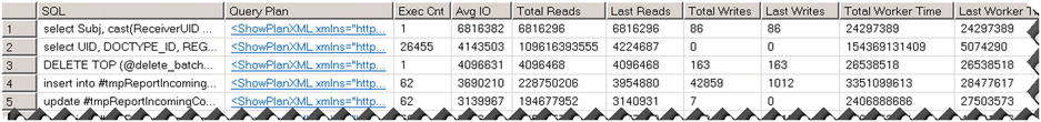
Figure 27-8. Query results
Unfortunately, sys.dm_exec_query_stats does not return any information for the queries, which do not have compiled plans cached. Usually, this is not an issue because our optimization targets are not only resource intensive, but they also frequently executed queries. Plans of those queries usually stay in cache due to their frequent re-use. However, SQL Server does not cache plans in the case of a statement-level recompile, therefore sys.dm_exec_query_stats misses them. You should use SQL Trace and/or Extended events to capture them. I usually start with queries from the sys.dm_exec_query_stats function output and crosscheck the optimization targets with Extended Events later.
![]() Note Query plans can be removed from the cache and, therefore, not included in the sys.dm_exec_query_stats results in cases of a SQL Server restart, memory pressure, and recompilations due to a statistics update and in a few other cases. It is beneficial to analyze the creation_time and last_execution_time columns in addition to the number of executions.
Note Query plans can be removed from the cache and, therefore, not included in the sys.dm_exec_query_stats results in cases of a SQL Server restart, memory pressure, and recompilations due to a statistics update and in a few other cases. It is beneficial to analyze the creation_time and last_execution_time columns in addition to the number of executions.
SQL Server 2008 and above provides stored procedure-level execution statistics with the sys.dm_exec_procedure_stats view. It provides similar metrics with sys.dm_exec_query_stats, and it can be used to determine the most resource-intensive stored procedures in the system. Listing 27-6 shows a query that returns the 50 most I/O intensive stored procedures, which have plan cached at the moment of execution.
Listing 27-6. Using sys.dm_exec_procedure_stats
select top 50
        db_name(ps.database_id) as [DB]
        ,object_name(ps.object_id, ps.database_id) as [Proc Name]
        ,ps.type_desc as [Type]
        ,qp.query_plan as  [Plan]
        ,ps.execution_count as [Exec Count]
        ,(ps.total_logical_reads + ps.total_logical_writes) /
                ps.execution_count as [Avg IO]
        ,ps.total_logical_reads as [Total Reads]
        ,ps.last_logical_reads as [Last Reads]
        ,ps.total_logical_writes as [Total Writes]
        ,ps.last_logical_writes as [Last Writes]
        ,ps.total_worker_time as [Total Worker Time]
        ,ps.last_worker_time as [Last Worker Time]
        ,ps.total_elapsed_time / 1000 as [Total Elapsed Time]
        ,ps.last_elapsed_time / 1000 as [Last Elapsed Time]
        ,ps.last_execution_time as [Last Exec Time]
from
        sys.dm_exec_procedure_stats ps with (nolock)
                cross apply sys.dm_exec_query_plan(ps.plan_handle) qp
order by
        [Avg IO] desc
option (recompile)
There are plenty of tools available on the market to help you automate the data collection and analysis process including the SQL Server Management Data Warehouse. All of them help you to achieve the same goal and find optimization targets in the system.
Finally, it is worth mentioning that the Data Warehouse and Decision Support Systems usually play under different rules. In those systems, it is typical to have I/O intensive queries that scan large amounts of data. Performance tuning of such systems can require different approaches than those found in OLTP environments, and they often lead to database schema changes rather than index tuning.
Memory-Related Wait Types
The RESOURCE_SEMAPHORE wait type indicates the wait for the query memory grant. As already discussed, every query in SQL Server requires some memory to execute. When there is no memory available, SQL Server places a query in one of three queues, based on the memory grant size, where it waits until memory becomes available. A high percentage of RESOURCE_SEMAPHORE waits indicate that SQL Server does not have enough memory to fulfill all memory grant requests.
You can confirm the problem by looking at the Memory Grants Pending performance counter in the Memory Manager Object. This counter shows the number of queries waiting for memory grants. Ideally, the counter value should be zero all the time. You can also look at the sys.dm_exec_query_memory_grants view, which provides information about memory grant requests, both pending and outstanding.
Obviously, one of the ways to address this issue is to reduce the memory grant size for the queries. You can optimize or simplify the queries in a way that removes memory-intensive operators, hashes, and sorts, for example, from the execution plan. You can obtain the query plan and text from the sys.dm_exec_query_memory_grants view directly, as shown in Listing 27-7. It is also possible, however, to take a general approach and focus on non-optimized queries. General query optimization reduces the load on the system, which leaves more server resources available.
Listing 27-7. Obtaining query information from the sys.dm_exec_query_memory_grants view
select
        mg.session_id
        ,t.text as [SQL]
        ,qp.query_plan as [Plan]
        ,mg.is_small
        ,mg.dop
        ,mg.query_cost
        ,mg.request_time
        ,mg.required_memory_kb
        ,mg.requested_memory_kb
        ,mg.wait_time_ms
        ,mg.grant_time
        ,mg.granted_memory_kb
        ,mg.used_memory_kb
        ,mg.max_used_memory_kb
from
        sys.dm_exec_query_memory_grants mg with (nolock)
                cross apply sys.dm_exec_sql_text(mg.sql_handle) t
                cross apply sys.dm_exec_query_plan(mg.plan_handle) as qp
option (recompile)
CXMEMTHREADis another memory-related wait type that you can encounter in systems. These waits occur when multiple threads are trying to allocate memory from HEAP simultaneously. You can often observe a high percentage of these waits in systems with a large number of ad-hoc queries where SQL Server constantly allocates and de-allocates plan cache memory. Enabling the Optimize for Ad-hoc Workloads configuration setting can help address this problem if plan cache memory allocation is the root-cause.
SQL Server has three types of memory objects that use HEAP memory. Some of them are created globally on the server scope. Others are partitioned on a per-NUMA Node or per-CPU basis. You can use startup trace flag T8048 to switch per-NUMA Node to per-CPU partitioning, which can help reduce CXMEMTHREAD waits at cost of extra memory usage.
![]() Note You can read more about Non-uniform Memory Access (NUMA) architecture at: http://technet.microsoft.com/en-us/library/ms178144.aspx.
Note You can read more about Non-uniform Memory Access (NUMA) architecture at: http://technet.microsoft.com/en-us/library/ms178144.aspx.
Listing 27-8 shows you how to analyze memory allocations of memory objects. You may consider applying the T8048 trace flag if top memory consumers are per-NUMA Node partitioned, and you can see a large percentage of CXMEMTHREAD waits in the system. This is especially important in the case of servers with more than eight CPUs per-NUMA Node, where SQL Server 2008 and above have known issues of per-NUMA Node memory object scalability.
Listing 27-8. Analyzing memory object partitioning and memory usage
select
        type
        ,pages_in_bytes
        , case
                when (creation_options & 0x20 = 0x20)
                        then 'Global PMO. Cannot be partitioned by CPU/NUMA Node. T8048 not applicable.'
                when (creation_options & 0x40 = 0x40)
                        then 'Partitioned by CPU. T8048 not applicable.'
                when (creation_options & 0x80 = 0x80)
                        then 'Partitioned by Node. Use T8048 to further partition by CPU.'
                else
                        'Unknown'
        end as [Partitioning Type]
from
        sys.dm_os_memory_objects
order by
        pages_in_bytes desc
![]() Note You can read an article published by the Microsoft CSS Team which explains how to debug CXMEMTHREAD wait types at: http://blogs.msdn.com/b/psssql/archive/2012/12/20/how-it-works-cmemthread-and-debugging-them.aspx.
Note You can read an article published by the Microsoft CSS Team which explains how to debug CXMEMTHREAD wait types at: http://blogs.msdn.com/b/psssql/archive/2012/12/20/how-it-works-cmemthread-and-debugging-them.aspx.
As strange as it sounds, low CPU load on a server is not necessarily a good sign. It indicates that the server is under-utilized. Even though under-utilization leaves systems with room to grow, it increases the IT infrastructure and operational costs—there are more servers to host and maintain. Obviously, high CPU load is not good either. Constant CPU pressure on SQL Server makes systems unresponsive and slow.
There are several indicators that can help you detect that a server is working under CPU pressure. These include a high percentage of SOS_SCHEDULER_YIELD waits, which occur when a worker is waiting in a runnable state. You can analyze the % Processor Time and Processor Queue Length performance counters and compare the signal and resource wait times in the sys.dm_os_wait_stats view, as shown in Listing 27-9. Signal waits indicate the waiting times for the CPU, while resource waits indicate the waiting times for resources, such as for pages from disk. Although Microsoft recommends that the signal wait type should not exceed 25 percent, I believe that 15-20 percent is a better target on busy systems.
Listing 27-9. Comparing signal and resource waits
select
        sum(signal_wait_time_ms) as [Signal Wait Time (ms)]
        ,convert(decimal(7,4), 100.0 * sum(signal_wait_time_ms) /
                sum (wait_time_ms)) as [% Signal waits]
        ,sum(wait_time_ms - signal_wait_time_ms) as [Resource Wait Time (ms)]
        ,convert(decimal(7,4), 100.0 * sum(wait_time_ms - signal_wait_time_ms) /
                sum (wait_time_ms)) as [% Resource waits]
from
        sys.dm_os_wait_stats with (nolock)
option (recompile)
Plenty of factors can contribute to CPU load in a system, and bad T-SQL code is at the top of the list. Imperative processing, cursors, XQuery, multi-statement user-defined functions and complex calculations are especially CPU-intensive.
The process of detecting the most CPU-intensive queries is very similar to that for detecting non-optimized queries. You can use the sys.dm_exec_query_stats view, as was shown in Listing 27-5. You can sort the data by the total_worker_time column, which detects the most CPU-intensive queries with plans currently cached. Alternatively, you can use SQL Trace and Extended Events, filtering data by CPU time rather than by I/O metrics.
![]() Note Both Extended Events and especially SQL Trace introduce additional overhead on the server and are not always the best option if CPU load is very high. At a bare minimum, avoid SQL Trace and use Extended Events if this is the case.
Note Both Extended Events and especially SQL Trace introduce additional overhead on the server and are not always the best option if CPU load is very high. At a bare minimum, avoid SQL Trace and use Extended Events if this is the case.
Constant recompilation is another source of CPU load. You can check the Batch Requests/Sec, SQL Compilations/Sec, and SQL Recompilations/Sec performance counters and calculate plan reuse with the following formula:
Plan Reuse = (Batch Requests/Sec - (SQL Compilations/Sec - SQL Recompilations/Sec)) / Batch Requests/Sec
Low plan reuse in OLTP systems indicates heavy Ad-Hoc activity and often requires code refactoring and parameterization of queries. However, non-optimized queries are still the major contributor to CPU load. With non-optimized queries, SQL Server processes a large amount of data, which burns CPU cycles regardless of other factors. In most cases, query optimization reduces the CPU load in the system.
Obviously, the same is true for bad T-SQL code. You should reduce the amount of imperative data processing, avoid multi-statement functions, and move calculations and XML processing to the application side if at all possible.
Parallelism
Parallelism is perhaps one of the most confusing aspects of troubleshooting. It exposes itself with the CXPACKET wait type, which often can be seen in the list of top waits in the system. The CXPACKET wait type, which stands for Class eXchange, occurs when parallel threads are waiting for other threads to complete their execution.
Let’s consider a simple example and assume that we have a parallel plan with two threads followed by the Exchange/Repartition Streams operator. When one parallel thread finishes its work, it waits for another thread to complete. The waiting thread does not consume any CPU resources; it just waits, generating the CXPACKET wait type.
The CXPACKET wait type merely indicates that there is parallelism in the system and, as usual, it fits into the “It Depends” category. It is beneficial when large and complex queries utilize parallelism, because it can dramatically reduce their response time. However, there is always overhead associated with parallelism management and Exchange operators. For example, if a serial plan finishes in 1 second on a single CPU, the execution time of the parallel plan that uses two CPUs would always exceed 0.5 seconds. There is always extra time required for parallelism management. Even though the response (elapsed) time of the parallel plan would be smaller, the CPU time will always be greater than in the case of the serial plan. You want to avoid such overhead when a large number of OLTP queries are waiting for the available CPU to execute. A high percent of SOS_SCHEDULER_YIELD and CXPACKET waits is a sign of such a situation.
One common misconception suggests that you completely disable parallelism in the case of a large percentage of CXPACKET waits in OLTP systems and set the server-level MAXDOP setting to 1. However, this is not the right way to deal with parallelism waits. You need to investigate the root-cause of parallelism in the OLTP system and analyze why SQL Server generates parallel execution plans. In most cases, it occurs due to complex and/or non-optimized queries. Query optimization simplifies execution plans and removes parallelism.
Moreover, any OLTP system has some legitimate complex queries that would benefit from parallelism. It is better to increase the Cost Threshold for Parallelism configuration option rather than to disable parallelism by setting the MAXDOP setting to 1. This would allow you to utilize parallelism with complex and expensive queries while keeping low-cost OLTP queries running serially.
There is no generic advice for how the Cost Threshold for Parallelism value needs to be set. By default, it is set to five, which is very low nowadays. You should analyze the activity and cost of the queries in your system to find the optimal value for this setting. Check the cost of the queries that you want to run serially and in parallel, and adjust the threshold value accordingly.
![]() Tip You can check the plan cost for a query in the properties of the root (top) operator in the execution plan.
Tip You can check the plan cost for a query in the properties of the root (top) operator in the execution plan.
Speaking of the MAXDOP setting, as general advice, it should not exceed the number of logical CPUs per hardware NUMA node. However, in some Data Warehouse/Decision Support Systems, you can consider using a MAXDOP setting that exceeds this number. Again, you should analyze and test your workload to find the most optimal value for this setting.
Locking and Blocking
Excessive locking and blocking issues in a system presents various LCK_M_* wait types. Each lock type has its own corresponding wait type. For example, LCK_M_U indicates update (U) lock waits, which can be a sign of non-optimized data modification queries.
We have already covered how to troubleshoot locking and blocking issues in a system. You need to detect what processes participated in the blocking chain with the Blocked Process Report, Deadlock Graph events, and sys.dm_tran_locks view and find the root-cause of the blocking. In most cases, it happens due to non-optimized queries.
In rare cases, SQL Server can experience worker thread starvation, a situation where there are no available workers to assign to new tasks. One scenario when this can happen is when a task acquires and holds a lock on a critical resource that is blocking a large number of other tasks/workers, which stays in a suspended state. When the number of workers in the system reaches the Maximum Worker Thread configuration setting, SQL Server is not able to create new workers, and new tasks remain unassigned, generating THREADPOOL waits.
Blocking is not the only reason why this situation could occur. It is also possible to reach the limit of worker threads in systems with heavy concurrent workload from a large number of users.
As usual, you need to find the root-cause of the problem. While it is possible to increase the Maximum Worker Thread number in the SQL Server configuration, this may or may not help. For example, in the blocking scenario described above, there is a good chance that newly created workers will be blocked in the same way as existing ones. It is better to investigate the root-cause of the blocking problem and address it instead.
You can check a blocking condition and locate the blocking session by analyzing the results of the sys.dm_os_waiting_tasks or sys.dm_exec_requests views. Listing 27-10 demonstrates the first approach. Keep in mind that the sys.dm_exec_requests view does not show tasks that do not have workers assigned waiting with the THREADPOOL wait type.
Listing 27-10. Using sys.dm_os_waiting_tasks
select
        wt.session_id
        ,wt.wait_type
        ,wt.wait_duration_ms
        ,wt.blocking_session_id
        ,wt.resource_description
from
        sys.dm_os_waiting_tasks wt with (nolock)
order by
        wt.wait_duration_ms desc
option (recompile)
As you can see in Figure 27-9, the ID of the blocking session is 51.
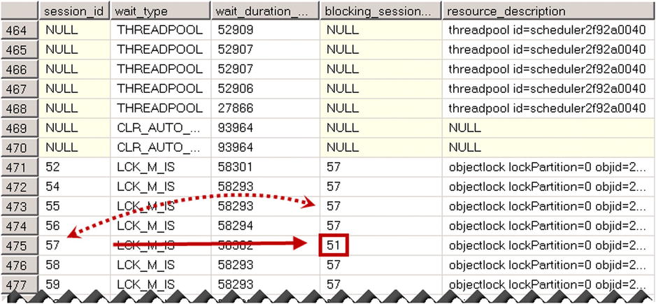
Figure 27-9. Sys.dm_os_waiting_tasks result
For the next step, you can use the sys.dm_exec_sessions and sys.dm_exec_connections views to get information about the blocking session, as shown in Listing 27-11. You can troubleshoot why the lock is held and/or terminate the session with the KILL command if needed.
Listing 27-11. Getting information about a blocking session
select
        ec.session_id
        ,s.login_time
        ,s.host_name
        ,s.program_name
        ,s.login_name
        ,s.original_login_name
        ,ec.connect_time
        ,qt.text as [SQL]
from
        sys.dm_exec_connections ec with (nolock)
                join sys.dm_exec_sessions s with (nolock) on
                        ec.session_id = s.session_id
                cross apply
                        sys.dm_exec_sql_text(ec.most_recent_sql_handle) qt
where
        ec.session_id = 51 -- session id of the blocking session
option (recompile)
![]() Note Worker thread starvation may prevent any connections to the server. In that case, you need to use Dedicated Admin Connection (DAC) for troubleshooting. We will discuss DAC later in this chapter.
Note Worker thread starvation may prevent any connections to the server. In that case, you need to use Dedicated Admin Connection (DAC) for troubleshooting. We will discuss DAC later in this chapter.
It is worth mentioning that even though increasing the Maximum Worker Thread setting does not necessarily solve the problem, it is always worth upgrading to a 64-bit version of Windows and SQL Server. A 64-bit version of SQL Server has more worker threads available by default, and it can utilize more memory for query grants and other components. It reduces memory grant waits, makes SQL Server more efficient and, therefore, allows tasks to complete execution and frees up workers faster.
Workers, however, consume memory, which reduces the amount of memory available to other SQL Server components. This is not usually an issue unless SQL Server is running on a server with very little physical memory available. You should consider adding more memory to the server if this is the case. After all, it is a cheap solution nowadays.
ASYNC_NETWORK_IO Waits
The ASYNC_NETWORK_IO wait type occurs when SQL Server generates data faster than the client application consumes it. While this could be a sign of non-sufficient network throughput, in a large number of cases ASYNC_NETWORK_IO waits are accumulated due to incorrect or inefficient client code.
One such example is reading an excessive amount of data from the server. The client application reads unnecessary data or, perhaps, performs client-side filtering, which adds extra load and exceeds network throughput.
Another pattern includes reading and simultaneous processing of the data, as shown in Listing 27-12. The client application consumes and processes rows one-by-one, keeping SqlDataReader open. Therefore, the worker waits for the client to consume all rows generating the ASYNC_NETWORK_IO wait type.
Listing 27-12. Reading and processing of the data: Incorrect implementation
using (SqlConnection connection = new SqlConnection(connectionString))
{
        SqlCommand command = new SqlCommand(cmdText, connection);
        connection.Open();

        using (SqlDataReader reader = command.ExecuteReader())
        {
                while (reader.Read())
                {
                        ProcessRow((IDataRecord)reader);
                }
        }
}
The correct way of handling such a situation is by reading all rows first as fast as possible and processing them after all rows have been read. Listing 27-13 illustrates this approach.
Listing 27-13. Reading and processing of the data: Correct implementation
List<Orders> orderRows = new List<Orders>();

using (SqlConnection connection = new SqlConnection(connectionString))
{
        SqlCommand command = new SqlCommand(cmdText, connection);
        connection.Open();

        using (SqlDataReader reader = command.ExecuteReader())
        {
                while (reader.Read())
                {
                        orderRows.Add(ReadOrderRow((IDataRecord)reader));
                }
        }
}

ProcessAllOrderRows(orderRows);
![]() Note You can easily duplicate such behavior by running a test in Management Studio connecting to a SQL Server instance locally. It would use the Shared Memory protocol without any network traffic involved. You can clear wait statistics on the server using the DBCC SQLPERF ('sys.dm_os_wait_stats', CLEAR) command, and run a select statement that reads a large amount of data displaying it in the result grid. If you checked the wait statistics after execution, you would see a large number of ASYNC_NETWORK_IO waits due to the slow grid performance, even though Management Studio is running locally on a SQL Server box. After that, repeat the test with the Discard Results After Execution configuration setting enabled. You should see the ASYNC_NETWORK_IO waits disappear.
Note You can easily duplicate such behavior by running a test in Management Studio connecting to a SQL Server instance locally. It would use the Shared Memory protocol without any network traffic involved. You can clear wait statistics on the server using the DBCC SQLPERF ('sys.dm_os_wait_stats', CLEAR) command, and run a select statement that reads a large amount of data displaying it in the result grid. If you checked the wait statistics after execution, you would see a large number of ASYNC_NETWORK_IO waits due to the slow grid performance, even though Management Studio is running locally on a SQL Server box. After that, repeat the test with the Discard Results After Execution configuration setting enabled. You should see the ASYNC_NETWORK_IO waits disappear.
You should check network performance and analyze the client code if you see a large percentage of ASYNC_NETWORK_IO waits in the system.
Allocation Map Contention and Tempdb load
Allocation map pagescontention exposes itself with PAGELATCH_* wait types. These wait types indicate contention on in-memory pages as opposed to PAGEIOLATCH wait types, which are I/O subsystem related.
![]() Note Latches are lightweight synchronization objects that protect the consistency of SQL Server internal data structures. For example, latches prevent multiple sessions from changing an in-memory data page simultaneously and corrupting it.
Note Latches are lightweight synchronization objects that protect the consistency of SQL Server internal data structures. For example, latches prevent multiple sessions from changing an in-memory data page simultaneously and corrupting it.
Coverage of latches is beyond the scope of this book. You can read more about latches and latch contention troubleshooting at: http://www.microsoft.com/en-us/download/details.aspx?id=26665.
Allocation map pages contention rarely happens in user databases unless the data is highly volatile. One example is a system that collects data from external sources with very high inserts and, therefore, pages and extents allocations rates. However, as we have already discussed, allocation map pages contention could become a major performance bottleneck in the case of tempdb.
When you see a large percentage of PAGELATCH waits, you should locate the resources where contention occurs. You can monitor the wait_resource column in the sys.dm_exec_requests or resource_description columns in the sys.dm_os_waiting_tasks view for corresponding wait types. The information in those columns includes the database id, file id, and page number. You can reduce allocation map contention in the corresponding database by moving objects that lead to the contention to another filegroup with a larger number of data files.
![]() Tip You can move objects by performing an index rebuild in the new filegroup. Make sure that all data files in the new filegroup were created with the same size and auto-growth parameters, which evenly balances write activity between them.
Tip You can move objects by performing an index rebuild in the new filegroup. Make sure that all data files in the new filegroup were created with the same size and auto-growth parameters, which evenly balances write activity between them.
Remember that moving LOB data requires extra steps, as we have already discussed in Chapter 15, “Data Partitioning.”
In the case of allocation map contention in tempdb (database id is 2), you can prevent mixed extents allocation with T1118 trace flag and create temporary objects in a way that allows their caching. We have already discussed this in detail in Chapter 12, “Temporary Tables.”
Other tempdb related performance counters, which can help you monitor its load, include Version Store Generation Rate (KB/S), Version Store Size (KB) in Transactions Object and Temp Table Creation Rate, and Active Temp Tables in a General Statistics Object. Those counters are most useful with the baseline, where they can show the trends of tempdb load.
Wrapping Up
Table 27-1 shows symptoms of the most common problems you will encounter in systems, and it illustrates the steps you can take to address these problems.
Table 27-1. Common problems, symptoms, and solutions
Problem |
Symptoms / Monitoring Targets |
Further Actions |
|---|---|---|
Overloaded I/O Subsystem |
PAGEIOLATCH, IO_COMPLETION, WRITELOG, LOGBUFFER, BACKUPIO waits sys.dm_io_virtual_file_stats stalls Low Page Life Expectancy, High Page Read/Sec, Page Write/Sec performance counters |
Check I/O subsystem configuration and throughput, especially in cases of non-data page I/O waits. Detect and optimize I/O intensive queries using sys.dm_exec_query_stats, SQL Trace, and Extended Events. |
CPU Load |
High CPU load, SOS_SCHEDULER_YIELD waits, high percentage of signal waits |
Possible non-efficient T-SQL code. Detect and optimize CPU intensive queries using sys.dm_exec_query_stats, SQL Trace, and Extended Events. Check recompilation and plan reuse in OLTP systems. |
Query Memory Grants |
RESOURCE_SEMAPHORE waits. Non-zero Memory Grants Pending value. Pending requests in sys.dm_exec_memory_grants. |
Detect and optimize queries that require large memory grants. Perform general query tuning. |
HEAP Memory Allocation contention |
CXMEMTHREAD waits |
Enable the “Optimize for Ad-hoc Workloads” configuration setting. Analyze what memory objects consume the most memory, and switch to per-CPU partitioning with the T8048 trace flag if appropriate. Apply the latest service pack. |
Parallelism in OLTP systems |
CXPACKET waits |
Find the root-cause of parallelism; most likely non-optimized or reporting queries. Perform query optimization for the non-optimized queries that should not have parallel plans. Tune and increase Cost Threshold for Parallelism value. |
Locking and Blocking |
LCK_M_* waits. Deadlocks. |
Detect queries involved in blocking with sys.dm_tran_locks, Blocking Process Report, and Deadlock Graph. Eliminate root-cause of blocking, most likely non-optimized queries or client code issues. |
ASYNC_NETWORK_IO waits |
ASYNC_NETWORK_IO waits, Network performance counters |
Check network performance. Review and refactor client code (loading excessive amount of data and/or loading and processing data simultaneously). |
Worker thread starvation |
THREADPOOL waits |
Detect and address root-cause of the problem (blocking and/or load). Upgrade to 64-bit version of SQL Server. Increasing Maximum Working Thread number may or may not help. |
Allocation maps contention |
PAGELATCH waits |
Detect resource that lead to contention using sys.dm_os_waiting_tasks and sys.dm_exec_requests. Add more data files. In the case of tempdb, use T1118 and utilize temporary object caching. |
This list is by no means complete, however it should serve as a good starting point.
![]() Note Read “SQL Server 2005 Performance Tuning using the Waits and Queues” whitepaper for more detail about wait statistics-based performance troubleshooting methodology. It is available for download at: http://technet.microsoft.com/en-us/library/cc966413.aspx. Even though this whitepaper was written to address SQL Server 2005, the information within it applies to any newer version of SQL Server.
Note Read “SQL Server 2005 Performance Tuning using the Waits and Queues” whitepaper for more detail about wait statistics-based performance troubleshooting methodology. It is available for download at: http://technet.microsoft.com/en-us/library/cc966413.aspx. Even though this whitepaper was written to address SQL Server 2005, the information within it applies to any newer version of SQL Server.
What to Do When the Server Is Not Responding
Situations where SQL Server stops responding, or where it is not accepting user requests, do not happen very often. Nevertheless, they do sometimes happen, and the first and most important rule is not to panic. SQL Server always treats data consistency as its top priority, and it is highly unlikely that something will happen to the data.
As a first step, you should validate that the problem is not infrastructure-related. You should check that the server and network are up and running and that the problem is not isolated to particular client workstation or subset of the network. It is entirely possible that the problem is not related to SQL Server at all. For example, changes in a firewall configuration or a network switch malfunction could block communication between SQL Server and client applications.
Next, you should check the SQL Server error log. Some conditions, for example prolonged worker thread starvation, leave error messages in the log, notifying the system administrator about the problem. Moreover, such conditions could introduce unhandled internal exceptions and mini-dumps. Unfortunately, there is no guarantee that SQL Server always recovers after such exceptions, and in some cases you will need to restart it. The key point with restart, however, is performing root-cause analysis of the problem. You need to analyze the error logs and default trace, do the research and, in some cases, open a support case with Microsoft to make sure that the problem is detected and addressed.
![]() Note Unhandled exceptions often occur due to bugs in SQL Server, which may already be fixed in the most recent service packs and cumulative updates. Consider applying them and open a support case with Microsoft CSS if this does not help.
Note Unhandled exceptions often occur due to bugs in SQL Server, which may already be fixed in the most recent service packs and cumulative updates. Consider applying them and open a support case with Microsoft CSS if this does not help.
You might need to connect to SQL Server for further troubleshooting. Fortunately, SQL Server 2005 introduced a special connection called Dedicated Admin Connection (DAC) that can be used for such a purpose. SQL Server reserves a private scheduler and a small amount of memory for DAC, which will allow you to connect even when SQL Server does not accept regular connections.
By default, DAC is available only locally. In some cases, when a server is completely overloaded, the operating system would not have adequate resources to handle user sessions, which prevents you from using DAC in local mode. You can change the configuration setting to allow a remote DAC connection with the code shown in Listing 27-14.
Listing 27-14. Enabling Remote Admin Connection
exec sp_configure 'remote admin connections', 1
go
reconfigure
go
You can connect to SQL Server with DAC by using the ADMIN: server name prefix in the Management Studio connection box or with the -A option in sqlcmd. Only members of the sysadmin server role are allowed to connect, and only one session can use a DAC connection at any point in time.
![]() Important You should use the connection dialog initiated from the Query Window when you use DAC from Management Studio. Object Explorer uses multiple database connections by design, and therefore it cannot use DAC. Make sure that Intellisense and other Management Studio plug-ins are disabled before you attempt this connection.
Important You should use the connection dialog initiated from the Query Window when you use DAC from Management Studio. Object Explorer uses multiple database connections by design, and therefore it cannot use DAC. Make sure that Intellisense and other Management Studio plug-ins are disabled before you attempt this connection.
A DAC connection can utilize a limited amount of resources, and it has a few restrictions on what operations can be done. For example, DAC does not support parallel query execution or backup/restore functions. It is designed for troubleshooting, and you should use DAC only for such a purpose.
We have already discussed worker thread starvation as one reason SQL Server may become unresponsive. Another possibility is run-away queries, which consume a major part of the resources on the server. You can detect such queries based on the sys.dm_exec_requests view, as shown in Listing 27-15.
Listing 27-15. Detecting run-away queries
select top 10
        er.session_id
        ,er.start_time
        ,er.cpu_time
        ,er.status
        ,er.command
        ,er.blocking_session_id
        ,er.wait_time
        ,er.wait_type
        ,er.last_wait_type
        ,er.logical_reads
        substring(qt.text, (er.statement_start_offset/2)+1,
                ((
                        case er.statement_end_offset
                                when -1 then datalength(qt.text)
                                else er.statement_end_offset
                        end - er.statement_start_offset)/2)+1) as SQL

from
        sys.dm_exec_requests er with (nolock)
                cross apply sys.dm_exec_sql_text(er.sql_handle) qt
order by cpu_time desc
option (recompile)
You can terminate a session with a run-away query using the KILL command. You should be careful, however, and analyze what the session is doing. SQL Server rolls back the active session transaction when you terminate it, which could be time and resource consuming in the case of heavy data modifications. It is entirely possible that allowing a session to finish a task is a faster and better option.
You can also consider using Resource Governor to prevent tasks from consuming all SQL Server resources. This could be especially useful if a server hosts multiple databases that belong to multiple systems. You can separate connections to different systems between resource pools, configured in a way that leaves some resources available for every system.
Working with Baseline
As you have already observed, I regularly mention the baseline in this chapter. Creating a baseline is an essential task for any database and IT professional. It allows you to be proactive and detect problems in the early stages before they become visible and impact system health and performance.
Many performance counters and metrics have very limited use by themselves. Some of them have a threshold or bad value that indicates a problem; however, a good value does not always guarantee that a system is healthy. It is always beneficial to look at dynamics and trends and monitor how values are changing.
Consider the Page Life Expectancy counter. The value of 10,000 is perfectly healthy for a server with 64GB of memory. However, if it were 50,000 last week, this would indicate that something has changed. Perhaps, the last deployment dropped some indexes or introduced non-optimized queries that triggered a heavy I/O load. Monitoring the Page Life Expectancy value over time allows you to be proactive and to start investigating and addressing the problem before it starts affecting other parts of the system.
Another good example is I/O subsystem performance. Every I/O subsystem has some breaking point when performance starts to drop exponentially with load increase. It is always beneficial to determine the limits before the initial deployment and to monitor how I/O load changes over time, making sure that there is still room to grow. The baseline will help you with monitoring and analysis.
![]() Tip You can use the SQLIO and SQLIOSIM utilities for stress testing of the I/O subsystem before the initial deployment. The SQLIO utility tests the general performance and throughput of the I/O subsystem. The SQLIOSIM utility emulates SQL Server I/O usage patterns. Both utilities are available for download from the Microsoft download center.
Tip You can use the SQLIO and SQLIOSIM utilities for stress testing of the I/O subsystem before the initial deployment. The SQLIO utility tests the general performance and throughput of the I/O subsystem. The SQLIOSIM utility emulates SQL Server I/O usage patterns. Both utilities are available for download from the Microsoft download center.
There are plenty of tools on the market that can help you automate baseline creation and monitoring. However, you can easily implement it manually by collecting and persisting metrics on a regular basis using various data management objects and Windows Performance Counters exposed through the sys.dm_os_performance_counters view. We have already discussed quite a few of them, and obviously you can expand upon this with other information as needed.
It is very important to capture the information for the system workload, which includes the number of connections, number of batches and transactions per second, size of the database, and other similar metrics. This will help you analyze trends, correlate workload with system load, and perform capacity analysis when needed.
It is also very beneficial to capture information about the performance of the system-critical parts of the code. Application developers can collect and persist the response time of the most critical queries and/or stored procedures, which will allow you to monitor trends, making sure that critical code performs satisfactorily all of the time.
Finally, creating a baseline is a very helpful first step in system troubleshooting. It helps you evaluate that you achieved desirable results and demonstrate them to management or customers.
Summary
Databases do not live in a vacuum. They are a part of a large ecosystem that includes various hardware and software components. Slowness and unresponsiveness of client applications are not necessarily database or SQL Server related. The root-cause of the problem can be anywhere in the system—from hardware misconfiguration to incorrect application code.
It is important to check the entire system infrastructure as an initial step in the troubleshooting process. This includes the performance characteristics of the hardware, network topology and throughput, operating system and SQL Server configuration, processes, and databases running on the server.
SQL Server consists of five major components including the protocol layer, query processor, storage engine, utilities, and SQL Server Operating System (SQLOS). SQLOS is the layer between Windows and all other SQL Server components, and it is responsible for scheduling, resource management, and several other low-level tasks.
SQLOS creates a number of schedulers equal to the number of logical processors in the system. Every scheduler is responsible for managing a set of workers that perform a job. Every task is assigned to one or more workers for the duration of the execution.
Tasks stay in one of three major states during execution: RUNNING (currently executing on scheduler), RUNNABLE (waiting for scheduler to execute), and SUSPENDED (waiting for the resource). SQL Server tracks the cumulative waiting time for the different types of waits and exposes this information to the users. Wait Statistics Analysis is a common performance troubleshooting technique that analyzes top system wait types and eliminates the root-causes of waits.
It is essential that you create a baseline by collecting and monitoring various performance and load metrics in the system. A baseline helps you to be proactive in detecting and resolving problems in the early stages before they start affecting the users. It shows how system behavior and load changes over time, which helps in capacity analysis and prevents the situation where a system outgrows the hardware.