![]()
Introduction to Columnstore Indexes
Columnstore indexes are Enterprise Edition feature, introduced in SQL Server 2012. They are part of the new family of technologies called xVelocity, which optimizes the performance of analytic queries that scan and aggregate large amounts of data.
Columnstore indexes use a different storage format for data, storing compressed data on a per-column rather than a per-row basis. This storage format benefits query processing in a Data Warehousing environment where, although queries typically read a very large number of rows, they work with just a subset of the columns from a table.
Design and implementation of Data Warehouse systems is a very complex process that is not covered in this book. This chapter, however, will reference common database design patterns frequently encountered in such systems. Moreover, it will provide an overview of columnstore indexes and their storage format, discuss batch-mode data processing, and outline several tips that can improve the performance of Data Warehouse solutions.
Data Warehouse Systems Overview
Data Warehouse systems provide the data that is used for analysis, reporting, and decision support purposes. In contrast to OLTP (Online Transactional Processing) systems, which are designed to support operational activity and which process simple queries in short transactions, Data Warehouse systems handle complex queries that usually perform aggregations and process large amounts of data.
For example, consider a company that sells articles to customers. A typical OLTP query from the company’s Point-of-Sale (POS) system might have the following semantic: Provide a list of orders that were placed by this particular customer this month. Alternatively, a typical query in a Data Warehouse system might read as follows: Provide the total amount of sales year to date, grouping the results by article categories and customer regions.
There are other differences between Data Warehouse and OLTP systems. Data in OLTP systems is usually volatile. Such systems serve a large number of requests simultaneously, and they often have a performance SLA associated with the customer-facing queries. Alternatively, the data in Data Warehouse systems is relatively static and is often updated based on a set schedule, such as at nights or during weekends. Those systems usually serve a small number of customers, typically business analysts, managers, and executives who can accept the longer execution time of the queries due to the amount of data that needs to be processed.
![]() Note To put things into perspective, the response time of the short OLTP queries usually needs to be in the milliseconds range. However, for complex Data Warehouse queries, a response time in seconds or even minutes is often acceptable.
Note To put things into perspective, the response time of the short OLTP queries usually needs to be in the milliseconds range. However, for complex Data Warehouse queries, a response time in seconds or even minutes is often acceptable.
The majority of companies start by designing or purchasing an OLTP system that supports the operational activities of the business. Reporting and analysis is initially accomplished based on OLTP data; however, as the business grows, that approach becomes more and more problematic. Database schema in OLTP systems rarely suit reporting purposes. Reporting activity adds load to the server and degrades the performance of and the customer experience in the system.
Data partitioning can help address some of these issues; however, there are limits on what can be achieved with such an approach. At some point, the separation of operational and analysis data becomes the only option that can guarantee the acceptable performance of both solutions.
![]() Note While you can technically separate OLTP and Data Warehouse data into different tables in the same database or in different databases running on the same SQL Server, it is rarely enough. The Data Warehouse workload is usually processing a large amount of data, and this adds a heavy load on the I/O subsystem and constantly flushes the content of the buffer pool. All of this negatively affects the performance of an OLTP system. It is better to deploy the Data Warehouse database to a separate server.
Note While you can technically separate OLTP and Data Warehouse data into different tables in the same database or in different databases running on the same SQL Server, it is rarely enough. The Data Warehouse workload is usually processing a large amount of data, and this adds a heavy load on the I/O subsystem and constantly flushes the content of the buffer pool. All of this negatively affects the performance of an OLTP system. It is better to deploy the Data Warehouse database to a separate server.
OLTP systems usually become the source of the data for Data Warehouses. The data from OLTP systems is transformed and loaded into a Data Warehouse with ETL(Extract Transform and Load) processes. This transformation is key here; that is, database schemas in OLTP and Data Warehouse systems do not and should not match.
A typical Data Warehouse database consists of several dimensions tables and one or a few facts tables. Facts tables store facts or measures of the business, while dimensions tables store the attributes or properties of facts. In our Point-of-Sale system, the information relating to sales becomes facts while the list of articles, customers, and branch offices become dimensions in the model.
Large facts tables can store millions or even billions of rows and use terabytes of disk space. Dimensions, on the other hand, are significantly smaller.
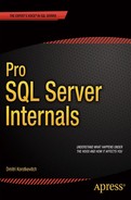
A typical Data Warehouse database design follows either a star or snowflake schema. A star schema consists of a facts table and a single layer of dimensions tables. A snowflake schema, on the other hand, normalizes dimensions tables even further.
Figure 34-1 shows an example of a star schema.
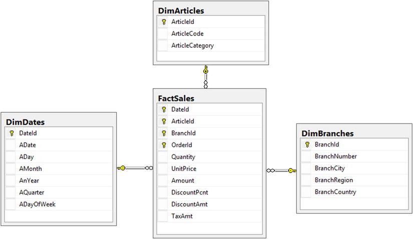
Figure 34-1. Star schema
Figure 34-2 shows an example of a snowflake schema for the same data model.
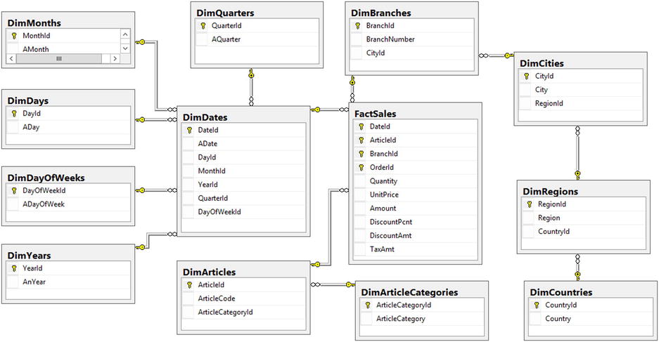
Figure 34-2. Snowflake schema
A typical query in Data Warehouse systems selects data from a facts table, joining it with one or more dimensions tables. SQL Server detects star and snowflake database schemas, and it uses a few optimization techniques to try and reduce the number of rows to scan and the amount of I/O required for a query. It pushes predicates towards the lowest operators in the execution plan tree, trying to evaluate them as early as possible and reducing the number of rows that need to be selected. Other optimizations include a cross join of dimensions tables and hash joins pre-filtering with Bitmap filters.
![]() Note Defining foreign key constraints between facts and dimensions tables helps SQL Server detect star and snowflake schemas more reliably. You may consider creating foreign key constraints using the WITH NOCHECK option if the overhead of constraint validation at the creation stage is unacceptable.
Note Defining foreign key constraints between facts and dimensions tables helps SQL Server detect star and snowflake schemas more reliably. You may consider creating foreign key constraints using the WITH NOCHECK option if the overhead of constraint validation at the creation stage is unacceptable.
Even with all optimizations, however, query performance in large Data Warehouses is not always sufficient. Scanning gigabytes or terabytes of data is time consuming even on today’s hardware. Part of the problem is the nature of query processing in SQL Server; that is, operators request and process rows one by one, which is not always efficient in the case of a large number of rows.
Some of these problems can be addressed with columnstore indexes and batch-mode data processing, which I will cover next.
Columnstore Indexes and Batch-Mode Processing Overview
As already mentioned, the typical Data Warehouse query joins facts and dimensions tables and performs some calculations and aggregations accessing just a subset of facts table’s columns. Listing 34-1 shows an example of such a query in the database that follows the star schema design pattern, as was shown in Figure 34-1.
Listing 34-1. Typical query in Data Warehouse environment
select a.ArticleCode, sum(s.Quantity) as [Units Sold]
from
        dbo.FactSales s join dbo.DimArticles a on
                s.ArticleId = a.ArticleId
        join dbo.DimDates d on
                s.DateId = d.DateId
where
        d.AnYear = 2014
group by
        a.ArticleCode
As you can see, this query needs to perform a scan of a large amount of data from the facts table; however, it uses just three table columns. With regular row-based processing, SQL Server accesses rows one by one, loading the entire row into memory, regardless of how many columns from the row are required.
You can reduce the storage size of the table and, therefore, the number of I/O operations by implementing page compression. However, page compression works in the scope of a single page. All pages will maintain a separate copy of the compression dictionary rather than use a single copy of dictionary for each table.
Finally, there is another, less obvious problem. Even though access to in-memory data is orders of magnitude faster than access to the data on disk, it is still slow as compared to CPU Cache access time. With row-based processing, SQL Server constantly reloads CPU Cache data with new rows copied from main memory. This overhead is usually not a problem with OLTP workload and simple queries; however, it becomes very noticeable with Data Warehouse queries that process millions or even billions of rows.
Column-Based Storage and Batch-Mode Execution
SQL Server addresses these problems with columnstore indexes and batch-mode execution. Columnstore indexes store data on a per-column rather than on a per-row basis. Figure 34-3 illustrates this approach.
Figure 34-3. Row-based and column-based storage
Data in columnstore indexes is heavily compressed using algorithms that provide significant space saving even when compared to page compression. Moreover, SQL Server can skip columns that are not requested by a query, and it does not load data from those columns into memory.
![]() Note We will compare the results of different compression methods in the next chapter.
Note We will compare the results of different compression methods in the next chapter.
The new data storage format of columnstore indexes allows SQL Server to implement a new batch-mode execution model that significantly reduces the CPU load and execution time of Data Warehouse queries. In this mode, SQL Server processes data in groups of rows, or batches, rather than one row at a time. The size of the batches varies to fit into the CPU cache, which reduces the number of times that the CPU needs to request external data from memory or other components. Moreover, the batch approach improves the performance of aggregations, which can be calculated on a per-batch rather than on a per-row basis.
In contrast to row-based processing where data values are copied between operators, batch-mode processing tries to minimize such copies by creating and maintaining a special bitmap that indicates if a row is still valid in the batch.
To illustrate this approach, let’s consider the following query:
select ArticleId, sum(Quantity)
from dbo.FactSales
where UnitPrice >=10.00
group by ArticleId
With regular, row-based processing, SQL Server scans a clustered index and applies a filter on every row. For rows that have UnitPrice >=10.00, it passes another row of two columns (ArticleId and Quantity) to the Aggregate operator. Figure 34-4 shows this process.
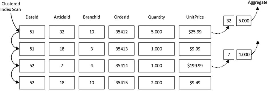
Figure 34-4. Row-mode processing
Alternatively, with batch-mode processing, the Filter operator would set an internal bitmap that shows the validity of the rows. A subsequent Aggregate operator would process the same batch of rows, ignoring non-valid ones. No data copying is involved. Figure 34-5 shows such an approach. It is also worth noting that only the ArticleId, Quantity, and UnitPrice columns would be loaded into the batch.
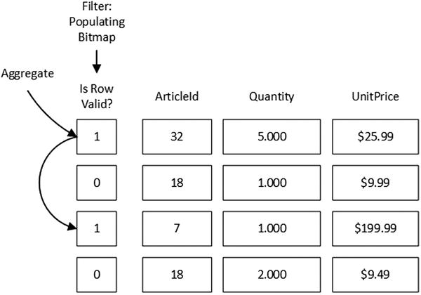
Figure 34-5. Batch-mode processing
![]() Note In a real system, SQL Server can push a predicate that evaluates if UnitPrice >=10 to the Columnstore Index Scan operator, preventing unnecessary rows from being loaded into the batch. However, let's assume that it is not the case in our example.
Note In a real system, SQL Server can push a predicate that evaluates if UnitPrice >=10 to the Columnstore Index Scan operator, preventing unnecessary rows from being loaded into the batch. However, let's assume that it is not the case in our example.
SQL Server handles parallelism in row- and batch-mode execution very differently. As you know, in row-based mode, an Exchange operator distributes rows between different parallel threads using one of the distribution algorithms available. However, after the distribution, a row never migrates from one thread to another until another Exchange operator gathers or repartitions the data.
Figure 34-6 illustrates this by demonstrating an Exchange operator that uses the Range redistribution method to distribute data to three parallel threads that perform Hash Joins. The first letter of a join key value would control to which thread row it is distributed and where it is processed.

Figure 34-6. Parallelism in row-mode processing
SQL Server takes a different approach with batch-mode processing. In that mode, every operator has a queue of work items (batches) to process. Worker threads from a shared pool pick items from queues and process them while migrating from operator to operator. Figure 34-7 illustrates this method.

Figure 34-7. Parallelism in batch-mode processing
One of the more common issues that increases the response time of parallel queries in row-mode execution is uneven data distribution. Exchange operators wait for all parallel threads to complete, thus the execution time depends on the slowest thread. Some threads have more work to do than others when data is unevenly distributed. Batch-mode execution eliminates such problems. Every thread picks up work items from the shared queue until the queue is empty.
Columnstore Indexes and Batch-Mode Execution in Action
Let’s look at several examples related to columnstore index behavior and performance. Listing 34-3 creates a set of tables for the database schema shown in Figure 34-1 and populates it with test data. As a final step, it creates a nonclustered columnstore index on the facts table. Based on the performance of your computer, it could take several minutes to complete.
Listing 34-3. Test database creation
create table dbo.DimBranches
(
        BranchId int not null primary key,
        BranchNumber nvarchar(32) not null,
        BranchCity nvarchar(32) not null,
        BranchRegion nvarchar(32) not null,
        BranchCountry nvarchar(32) not null
);

create table dbo.DimArticles
(
        ArticleId int not null primary key,
        ArticleCode nvarchar(32) not null,
        ArticleCategory nvarchar(32) not null
);

create table dbo.DimDates
(
        DateId int not null primary key,
        ADate date not null,
        ADay tinyint not null,
        AMonth tinyint not null,
        AnYear tinyint not null,
        AQuarter tinyint not null,
        ADayOfWeek tinyint not null
);

create table dbo.FactSales
(
        DateId int not null
                foreign key references dbo.DimDates(DateId),
        ArticleId int not null
                foreign key references dbo.DimArticles(ArticleId),
        BranchId int not null
                foreign key references dbo.DimBranches(BranchId),
        OrderId int not null,
        Quantity decimal(9,3) not null,
        UnitPrice money not null,
        Amount money not null,
        DiscountPcnt decimal (6,3) not null,
        DiscountAmt money not null,
        TaxAmt  money not null,
        primary key (DateId, ArticleId, BranchId, OrderId)
        with (data_compression = page)
);

;with N1(C) as (select 0 union all select 0) -- 2 rows
,N2(C) as (select 0 from N1 as T1 cross join N1 as T2) -- 4 rows
,N3(C) as (select 0 from N2 as T1 cross join N2 as T2) -- 16 rows
,N4(C) as (select 0 from N3 as T1 cross join N3 as T2) -- 256 rows
,N5(C) as (select 0 from N2 as T1 cross join N4 as T2) -- 1,024 rows
,IDs(ID) as (select ROW_NUMBER() over (order by (select NULL)) from N5)
,Dates(DateId, ADate)
as
(
        select ID, dateadd(day,ID,'2012-12-31')
        from IDs
        where ID <= 727
)
insert into dbo.DimDates(DateId, ADate, ADay, AMonth, AnYear
        ,AQuarter, ADayOfWeek)
        select DateID, ADate, Day(ADate), Month(ADate), Year(ADate)
                ,datepart(qq,ADate), datepart(dw,ADate)
        from Dates;


;with N1(C) as (select 0 union all select 0) -- 2 rows
,N2(C) as (select 0 from N1 as T1 cross join N1 as T2) -- 4 rows
,N3(C) as (select 0 from N2 as T1 cross join N2 as T2) -- 16 rows
,IDs(ID) as (select ROW_NUMBER() over (order by (select NULL)) from N3)
insert into dbo.DimBranches(BranchId, BranchNumber, BranchCity,
               BranchRegion, BranchCountry)
        select ID, convert(nvarchar(32),ID), 'City', 'Region', 'Country'
        from IDs
        where ID <= 13;

;with N1(C) as (select 0 union all select 0) -- 2 rows
,N2(C) as (select 0 from N1 as T1 cross join N1 as T2) -- 4 rows
,N3(C) as (select 0 from N2 as T1 cross join N2 as T2) -- 16 rows
,N4(C) as (select 0 from N3 as T1 cross join N3 as T2) -- 256 rows
,N5(C) as (select 0 from N4 as T1 cross join N2 as T2) -- 1,024 rows
,IDs(ID) as (select ROW_NUMBER() over (order by (select NULL)) from N5)
insert into dbo.DimArticles(ArticleId, ArticleCode, ArticleCategory)
        select ID, convert(nvarchar(32),ID), 'Category ' + convert(nvarchar(32),ID % 51)
        from IDs
        where ID <= 1021;

;with N1(C) as (select 0 union all select 0) -- 2 rows
,N2(C) as (select 0 from N1 as T1 cross join N1 as T2) -- 4 rows
,N3(C) as (select 0 from N2 as T1 cross join N2 as T2) -- 16 rows
,N4(C) as (select 0 from N3 as T1 cross join N3 as T2) -- 256 rows
,N5(C) as (select 0 from N4 as T1 cross join N4 as T2) -- 65,536 rows
,N6(C) as (select 0 from N5 as T1 cross join N4 as T2) -- 16,777,216 rows
,IDs(ID) as (select ROW_NUMBER() over (order by (select NULL)) from N6)
        insert into dbo.FactSales(DateId, ArticleId, BranchId, OrderId
                , Quantity, UnitPrice, Amount, DiscountPcnt, DiscountAmt, TaxAmt)
                select ID % 727 + 1, ID % 1021 + 1, ID % 13 + 1, ID
                        ,ID % 51 + 1, ID % 25 + 0.99
                        ,(ID % 51 + 1) * (ID % 25 + 0.99), 0, 0
                        ,(ID % 25 + 0.99) * (ID % 10) * 0.01
                from IDs;

create nonclustered columnstore index IDX_FactSales_ColumnStore
on dbo.FactSales(DateId, ArticleId, BranchId, Quantity, UnitPrice, Amount);
Let’s run several tests that select data from a facts table, joining it with one of the dimensions tables using different indexes and different degrees of parallelism, which leads to serial and parallel execution plans. I am running the queries in SQL Server 2012 and 2014 in 4-CPU virtual machines with 8GB of RAM allocated.
The first query shown in Listing 34-4 performs a Clustered Index Scan using a serial execution plan with row-mode execution.
Listing 34-4. Test query: Clustered Index Scan with MAXDOP=1
select a.ArticleCode, sum(s.Amount) as [TotalAmount]
from
        dbo.FactSales s with (index = 1) join dbo.DimArticles a on
                s.ArticleId = a.ArticleId
group by
        a.ArticleCode
option (maxdop 1)
Both SQL Server 2012 and 2014 produce identical execution plans, as shown in Figure 34-8.
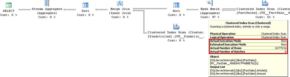
Figure 34-8. Execution plan with Clustered Index Scan and MAXDOP=1
Table 34-1 shows the execution statistics for the queries.
Table 34-1. Execution statistics: Clustered Index Scan and MAXDOP=1
Logical Reads |
CPU Time (ms) |
Elapsed Time (ms) |
|---|---|---|
50,760 |
5,644 |
5,944 |
In the next step, let’s remove the index hint and allow SQL Server to pick a columnstore index to access the data, still using the serial execution plan. The query is shown in Listing 34-5.
Listing 34-5. Test query: Columnstore Index Scan with MAXDOP=1
select a.ArticleCode, sum(s.Amount) as [TotalAmount]
from
        dbo.FactSales s join dbo.DimArticles a on
                s.ArticleId = a.ArticleId
group by
        a.ArticleCode
option (maxdop 1)
Again, both SQL Server 2012 and 2014 generated an identical execution plan, as shown in Figure 34-9. The plan utilizes a Columnstore Index Scan in row-mode execution.
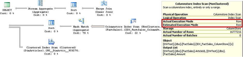
Figure 34-9. Execution plan with a Columnstore Index Scan and MAXDOP=1
Table 34-2 shows the execution statistics for the queries. As you can see, even with row-mode execution, the Columnstore Index Scan introduces more than a four times reduction in the number of reads, and it allowed the query to complete almost two times faster as compared to the Clustered Index Scan.
Table 34-2. Execution statistics: Columnstore Index Scan and MAXDOP=1
Logical Reads |
CPU Time (ms) |
Elapsed Time (ms) |
|---|---|---|
12,514 |
3,140 |
3,191 |
In the next group of tests, we will remove the MAXDOP hint, which will allow SQL Server to generate parallel execution plans. The first test would force SQL Server to use a Clustered Index Scan with the index hint, as shown in Listing 34-6.
Listing 34-6. Test query: Clustered Index Scan with parallel execution plan
select a.ArticleCode, sum(s.Amount) as [TotalAmount]
from
        dbo.FactSales s with (index = 1) join dbo.DimArticles a on
                s.ArticleId = a.ArticleId
group by
        a.ArticleCode
Figure 34-10 illustrates the execution plan for the query running in SQL Server 2012. Even though SQL Server generated a parallel execution plan, it used row-mode execution for all operators.
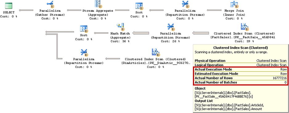
Figure 34-10. Execution plan with Clustered Index Scan in SQL Server 2012
If you ran the same query in SQL Server 2014, you would see different results, as shown in Figure 34-11. SQL Server still used row-mode execution during the Clustered Index Scan; however, Hash Join and Hash Aggregate operators are used in batch-mode execution.
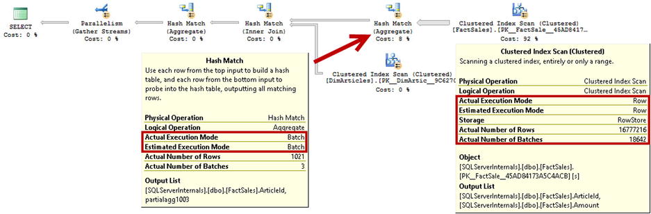
Figure 34-11. Execution plan with Clustered Index Scan in SQL Server 2014
![]() Note Batch-mode execution works only in parallel execution plans.
Note Batch-mode execution works only in parallel execution plans.
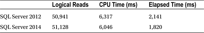
Table 34-3 shows the execution statistics for the queries in both SQL Server 2012 and 2014. As you can see, SQL Server 2014 performs slightly better due to batch-mode execution of the hash operators.
Table 34-3. Execution statistics: Clustered Index Scan and parallel execution plan
Finally, let’s remove the index hint and allow SQL Server to use a columnstore index and parallel execution plan. The query is shown in Listing 34-7.
Listing 34-7. Test query: Columnstore Index Scan with parallel execution plan
select a.ArticleCode, sum(s.Amount) as [TotalAmount]
from
        dbo.FactSales s join dbo.DimArticles a on
                s.ArticleId = a.ArticleId
group by
        a.ArticleCode
Figure 34-12 illustrates the execution plan of the query in SQL Server 2012. As you can see, it utilizes batch-mode execution. It is worth noting that the Exchange/Parallelism (Repartition Streams) operators in the execution plan do not move data between different threads, which you can see by analyzing the Actual Number of Rows operators’ property. SQL Server 2012 keeps them in the plan to support cases when a Hash Table spills to tempdb, which will force SQL Server to switch to row-mode execution.

Figure 34-12. Execution plan with a Columnstore Index Scan and batch-mode execution (SQL Server 2012)
Figure 34-13 shows the execution plan of the query in SQL Server 2014. As you can see, the execution plan is significantly simpler and does not include Parallelism/Exchange operators. SQL Server 2014 supports batch-mode execution even in cases of tempdb spills.
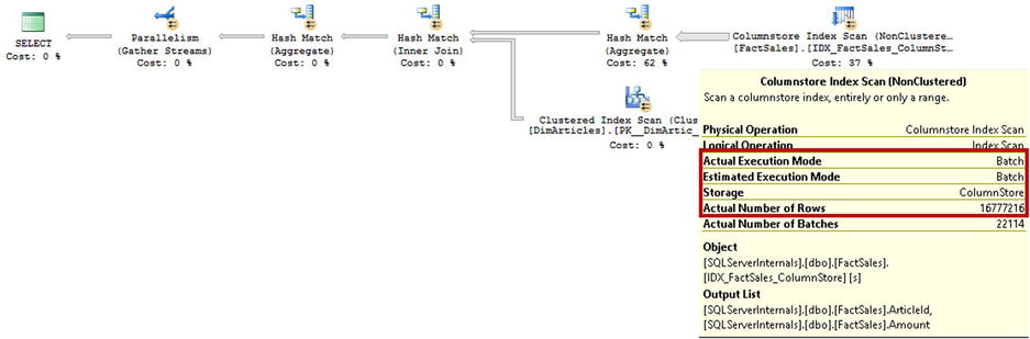
Figure 34-13. Execution plan with a Columnstore Index Scan and batch-mode execution (SQL Server 2014)
Table 34-4 illustrates the execution statistics for the queries. It is worth noting that, even though SQL Server 2014 performance improvements are marginal in batch-mode execution, this situation would change in the case of tempdb spills, when SQL Server 2012 would switch to row-mode execution.
Table 34-4. Execution statistics: Columnstore Index Scan and parallel execution plan
CPU Time (ms) |
Elapsed Time (ms) |
|
|---|---|---|
SQL Server 2012 |
703 |
246 |
SQL Server 2014 |
687 |
220 |
As you can see, columnstore indexes significantly reduce the I/O load in the system as well as the CPU and Elapsed time of the queries. The difference is especially noticeable in the case of batch-mode execution where the query ran almost ten times faster as compared to a row-mode clustered index scan.
There are two types of columnstore indexes available in SQL Server. SQL Server 2012 supports only nonclustered columnstore indexes. SQL Server 2014 supports clustered columnstore indexes in addition to nonclustered ones. Nevertheless, both clustered and nonclustered columnstore indexes share the same basic structure to store data.
![]() Note We will discuss clustered columnstore indexes in greater detail in Chapter 35, “Clustered Columnstore Indexes.”
Note We will discuss clustered columnstore indexes in greater detail in Chapter 35, “Clustered Columnstore Indexes.”
Nonclustered Columnstore Indexes
You can create a nonclustered columnstore index with the CREATE COLUMNSTORE INDEX command. You have already seen this command in action in Listing 34-3 in the previous section.
There are several things worth noting about this command. The CREATE COLUMNSTORE INDEX command looks like the regular CREATE INDEX command, and it allows you to specify the destination filegroup or partition schema for the index. However, it supports only two options during index creation such as, MAX_DOP and DROP_EXISTING.
A nonclustered columnstore index can include up to 1,024 non-sparse columns. Due to the nature of the index, it does not matter in what order the columns are specified; that is, data is stored on a per-column basis.
Similar to B-Tree nonclustered indexes, nonclustered columnstore indexes include a row-id, which is either a clustered index key value or the physical location of a row in a heap table. This behavior allows SQL Server to use the Columnstore Index Scan operation to perform Key Lookup afterwards. It is worth noting that columnstore indexes do not support a Seek operation because the data in those indexes is not sorted. We will talk about data storage in more detail shortly.
Listing 34-8 shows an example of a query that uses a Columnstore Index Scan with Key Lookup operators.
Listing 34-8. Query that triggers Key Lookup operation
select OrderId, Amount, TaxAmt
from dbo.FactSales
where ArticleId = -1
Figure 34-14 shows the execution plan for the query shown in Listing 34-8. It is worth noting that the OrderId column is included in the output list of the Columnstore Index Scan operator. That column has not been explicitly defined in the columnstore index; however, it is part of the clustered index key in the table.
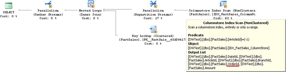
Figure 34-14. Execution plan for a query
Creation of a columnstore index is a very memory-intensive operation. When you create a columnstore index in SQL Server 2012, it requests a memory grant of a size that you can roughly estimate with the following formula:
Memory Grant Request (MB) =
         (4.2 * Number of columns in the index + 68) * (Degree of Parallelism) +
         (Number of text columns in the index * 34)
For example, the columnstore index created in Listing 34-3 requested a memory grant of 394MB in my environment, which is fairly close to the (4.2 * 7 (6 index columns + OrderId) + 68) * 4 = 390MB calculated with the formula. The size of the memory grant does not depend on the size of the table. As you will see later, SQL Server processes data in batches of about one million rows each.
The index creation process fails in cases of insufficient memory. There are two ways to solve this problem besides adding more memory to the server. The first is to reduce the degree of parallelism with the MAXDOP index option. While this option reduces the memory requirements for a query, it increases the index creation time proportionally to the decrease of DOP.
The second option is to change the REQUEST_MAX_MEMORY_GRANT_PERCENT property of the workload group in Resource Governor. By default, the size of the query memory grant is limited to 25 percent of the available memory. You can change it with the code shown in Listing 34-9 (assuming that you run a query under the default workload group). This approach allows you to increase the size of a memory grant; however, it would leave you with less available memory for other sessions during index creation. Do not forget to change the query memory grant, setting it back to the previous value afterwards.
Listing 34-9. Increasing the maximum memory grant size up to 50 percent of available memory
alter workload group [default] with (request_max_memory_grant_percent=50);
alter resource governor reconfigure;
![]() Note Coverage of the Resource Governor is outside of the scope of this book. You can read about the Resource Governor at: http://technet.microsoft.com/en-us/library/bb895232.aspx.
Note Coverage of the Resource Governor is outside of the scope of this book. You can read about the Resource Governor at: http://technet.microsoft.com/en-us/library/bb895232.aspx.
The index creation algorithm has been improved in SQL Server 2014. In contrast to SQL Server 2012, which uses a degree of parallelism that matches either server or index DOP option, SQL Server 2014 automatically adjusts the DOP based on available memory. This behavior decreases the chance that the index creation process will fail due to an out-of-memory condition.
Columnstore indexes have several restrictions that you need to remember. They cannot be defined as UNIQUE, cannot have sparse or computed columns, nor can they be created on an indexed view. Moreover, not all data types are supported. The list of unsupported data types includes the following:
- binary
- varbinary
- (n)text
- image
- (n)varchar(max)
- timestamp
- CLR types
- sql_variant
- xml
The following data types are not supported in SQL Server 2012; however, they are supported in SQL Server 2014:
- uniqueidentifier
- decimal and numeric with precision greater than 18 digits
- datetimeoffset with precision greater than 2
Another limitation of nonclustered columnstore indexes is that a table with such an index becomes read-only. You cannot change data in the table after the index is created. This limitation, however, is not as critical as it seems. Columnstore indexes are a Data Warehouse feature, and data is usually static in Data Warehouses. You can always drop a columnstore index before a data refresh and recreate it afterwards.
Tables with columnstore indexes support a partition switch, which is another option for importing data into the table. You can create a staging table using it as the target for data import, add a columnstore index to a staging table when the import is completed, and switch the staging table as the new partition to the main read-only table as the last step of the operation. Listing 34-10 shows an example of this.
Listing 34-10. Importing data into a table with a nonclustered columnstore index using a staging table and partition switch
create partition function pfFacts(int)
as range left for values (1,2,3,4,5);
go

create partition scheme psFacts
as partition pfFacts
all to ([FG2014]);
go

create table dbo.FactTable
(
        DateId int not null,
        ArticleId int not null,
        OrderId int not null,
        Quantity decimal(9,3) not null,
        UnitPrice money not null,
        Amount money not null,

        constraint PK_FactTable
        primary key clustered(DateId, ArticleId, OrderId)
        on psFacts(DateId)
)
go

;with N1(C) as (select 0 union all select 0) -- 2 rows
,N2(C) as (select 0 from N1 as T1 cross join N1 as T2) -- 4 rows
,N3(C) as (select 0 from N2 as T1 cross join N2 as T2) -- 16 rows
,N4(C) as (select 0 from N3 as T1 cross join N3 as T2) -- 256 rows
,N5(C) as (select 0 from N4 as T1 cross join N2 as T2) -- 1,024 rows
,IDs(ID) as (select ROW_NUMBER() over (order by (select NULL)) from N5)
insert into dbo.FactTable(DateId, ArticleId, OrderId, Quantity, UnitPrice, Amount)
        select ID % 4 + 1, ID % 100, ID, ID % 10 + 1, ID % 15 + 1 , ID % 25 + 1
        from IDs;
go

create nonclustered columnstore index IDX_FactTable_Columnstore
on dbo.FactTable(DateId, ArticleId, OrderId, Quantity, UnitPrice, Amount)
on psFacts(DateId)
go

create table dbo.StagingTable
(
        DateId int not null,
        ArticleId int not null,
        OrderId int not null,
        Quantity decimal(9,3) not null,
        UnitPrice money not null,
        Amount money not null,

        constraint PK_StagingTable
        primary key clustered(DateId, ArticleId, OrderId)
        on [FG2014],

        constraint CHK_StagingTable
        check(DateId = 5)
)
go


/*** Step 1: Importing data into a staging table ***/
;with N1(C) as (select 0 union all select 0) -- 2 rows
,N2(C) as (select 0 from N1 as T1 cross join N1 as T2) -- 4 rows
,N3(C) as (select 0 from N2 as T1 cross join N2 as T2) -- 16 rows
,N4(C) as (select 0 from N3 as T1 cross join N3 as T2) -- 256 rows
,N5(C) as (select 0 from N4 as T1 cross join N2 as T2) -- 1,024 rows
,IDs(ID) as (select ROW_NUMBER() over (order by (select NULL)) from N5)
insert into dbo.StagingTable(DateId, ArticleId, OrderId, Quantity, UnitPrice, Amount)
        select 5, ID % 100, ID, ID % 10 + 1, ID % 15 + 1 , ID % 25 + 1
        from IDs;
go


/*** Step 2: Creating nonclustered columstore index ***/
create nonclustered columnstore index IDX_StagingTable_Columnstore
on dbo.StagingTable(DateId, ArticleId, OrderId, Quantity, UnitPrice, Amount)
on [FG2014]
go

/*** Step 3: Switching a staging table as the new partition of the main table ***/
alter table dbo.StagingTable
switch to dbo.FactTable
partition 5;
![]() Tip You can use a partitioned view that combines data from updatable tables and read-only tables with columnstore indexes.
Tip You can use a partitioned view that combines data from updatable tables and read-only tables with columnstore indexes.
Finally, SQL Server 2014 introduces updateable clustered columnstore indexes, which we will discuss in the next chapter.
Each data column in columnstore indexes is stored separately in a set of structures called row groups. Each row group stores data for up to approximately one million or, to be precise, 2^20=1,048,576 rows. SQL Server tries to populate row groups completely during index creation, leaving the last row group partially populated. For example, if table has five million rows, SQL Server creates four row groups of 1,048,576 rows each and one row group with 805,696 rows.
![]() Note In practice, you can have more than one partially populated row group when multiple threads create columnstore indexes using a parallel execution plan. Each thread will work with its own subset of data, creating separate row groups in this scenario. Moreover, in the case of partitioned tables, each table partition has its own set of row groups.
Note In practice, you can have more than one partially populated row group when multiple threads create columnstore indexes using a parallel execution plan. Each thread will work with its own subset of data, creating separate row groups in this scenario. Moreover, in the case of partitioned tables, each table partition has its own set of row groups.
After row groups are built, SQL Server combines all column data on a per-row group basis and encodes and compresses them. The rows within a row group can be rearranged if that helps to achieve a better compression rate.
Column data within a row group is called a segment. SQL Server loads an entire segment to memory when it needs to access columnstore data.
Figure 34-15 illustrates the index creation process. It shows a columnstore index with four columns and three row groups. Two row groups are populated in full and the last one is partially populated.
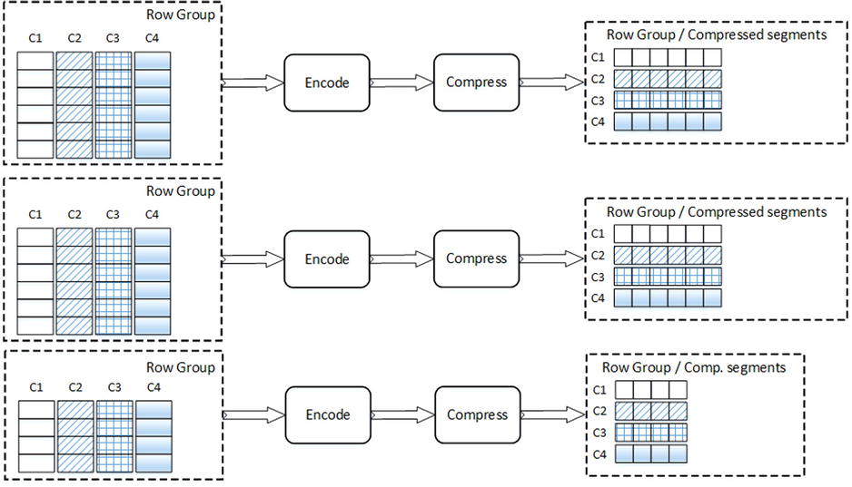
Figure 34-15. Building a columnstore index
During encoding, SQL Server replaces all values in the data with 64-bit integers using one of two encoding algorithms. The first algorithm, called dictionary encoding, stores distinct values from the data in a separate structure called a dictionary. Every value in a dictionary has a unique ID assigned. SQL Server replaces the actual value in the data with an ID from the dictionary.
SQL Server creates one primary dictionary, which is shared across all row groups that belong to the same index partition. Moreover, SQL Server can create one secondary dictionary that stores only the values from string columns per row group. The purpose of secondary dictionaries is to reduce memory requirements during index creation and scan operations.
Figure 34-16 illustrates dictionary encoding. For simplicity sake, it shows neither multiple row groups nor secondary dictionaries in order to focus on the main idea of the algorithm.

Figure 34-16. Dictionary encoding
The second type of encoding, called value-based encoding, is mainly used for numeric and integer data types that do not have enough duplicated values. With this condition, dictionary encoding is inefficient. The purpose of value-based encoding is to convert integer and numeric values to a smaller range of 64-bit integers. This process consists of the following two steps.
In the first step, numeric data types are converted to integers using the minimum positive exponent that allows this conversion. Such an exponent is called magnitude. For example, for a set of values such as 0.8, 1.24, and 1.1, the minimum exponent is 2, which represents a multiplier of 100. After this exponent is applied, values would be converted to 80, 124, and 110 respectively. The goal of this process is to convert all numeric values to integers.
Alternatively, for integer data types, SQL Server chooses the smallest negative exponent that can be applied to all values without losing their precision. For example, for the values 1340, 20, and 2,340, that exponent is -1, which represents a divider of 10. After this operation, the values would be converted to 134, 2, and 234 respectively. The goal of such an operation is to reduce the interval between the minimum and maximum values stored in the segment.
During the second step, SQL Server chooses the base value, which is the minimum value in the segment, and it subtracts it from all other values. This makes the minimum value in the segment 0.
Figure 34-17 illustrates the process of value-based encoding.
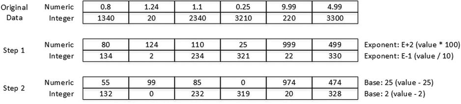
Figure 34-17. Value-based encoding
After encoding, SQL Server compresses the data and stores it as a LOB allocation unit. We have discussed how this type of data is stored in Chapter 1 “Data Storage Internals.”
Listing 34-11 shows a query that displays allocation units for the dbo.FactSales table.
Listing 34-11. dbo.FactSales table allocation units
select i.name as [Index], p.index_id
        ,p.partition_number as [Partition]
        ,p.data_compression_desc as [Compression]
        ,u.type_desc, u.total_pages
from
        sys.partitions p join sys.allocation_units u on
                p.partition_id = u.container_id
        join sys.indexes i on
                p.object_id = i.object_id and
                p.index_id = i.index_id
where
        p.object_id = object_id(N'dbo.FactSales')
As you can see in Figure 34-18, the columnstore index is stored as LOB_DATA. It is worth noting that this index has IN_ROW_DATA allocation units; however, these allocation units do not store any data. It is impossible to have LOB_DATA allocation in the index without an IN_ROW_DATA allocation present.

Figure 34-18. dbo.FactSales table allocation units
SQL Server provides two columnstore index-related data management views. Let’s look at them in depth.
The sys.column_store_segments view returns one row for each column per segment.
Listing 34-12 shows a query that returns information about the IDX_FactSales_ColumnStore columnstore index defined on dbo.FactSales table. There are a couple of things that you should note here. First, the sys.column_store_segments view does not return the object_id or index_id of the index. This is not a problem because a table can have only one columnstore index defined. However, you need to use the sys.partitions view to obtain the object_id when it is required.
Listing 34-12. Examining the sys.column_store_segments view
select p.partition_number as [partition], c.name as [column]
        ,s.column_id, s.segment_id, p.data_compression_desc as [compression]
        ,s.version, s.encoding_type, s.row_count, s.has_nulls, s.magnitude
        ,s.primary_dictionary_id, s.secondary_dictionary_id, s.min_data_id
        ,s.max_data_id, s.null_value
        ,convert(decimal(12,3),s.on_disk_size / 1024. / 1024.)  as [Size MB]
from
        sys.column_store_segments s join sys.partitions p on
                p.partition_id = s.partition_id
        join sys.indexes i on
                p.object_id = i.object_id
        left join sys.index_columns ic on
                i.index_id = ic.index_id and
                i.object_id = ic.object_id and
                s.column_id = ic.index_column_id
        left join sys.columns c on
                ic.column_id = c.column_id and
                ic.object_id = c.object_id
where
        i.name = 'IDX_FactSales_ColumnStore'
order by
        p.partition_number, s.segment_id, s.column_id
Second, like regular B-Tree indexes, nonclustered columnstore indexes include a row-id, which is either the address of a row in a heap table or a clustered index key value. In the latter case, all columns from the clustered index are included in the columnstore index, even when you do not explicitly define them in the CREATE COLUMNSTORE INDEX statement. However, these columns would not exist in the sys.index_columns view, and you need to use an outer join when you want to obtain the column name.
Figure 34-19 shows the partial output of a query from Listing 34-12. Column 8, which does not have column name displayed, represents the OrderId column, which is a part of the clustered index and has not been explicitly defined in the columnstore index.
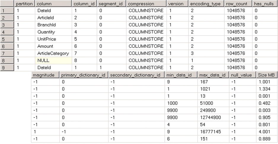
Figure 34-19. sys.column_store_segments output
The columns in the output represent the following:
- column_id is the ID of a column in the index, which you can join with the sys.index_columns view. As you have seen, only columns that are explicitly included in an index have corresponding sys.index_columns rows.
- partition_id references the partition to which a row group (and, therefore, a segment) belongs. You can use it in a join with sys.partitions view to obtain object_id of the index.
- segment_id is the ID of the segment, which is basically the ID of a row group. The first segment in partition has ID of 0.
- version represents a columnstore segment format. Both, SQL Server 2012 and 2014 return 1 as its value.
- encoding_type represents the encoding used for this segment. It can have one of the following four values:
- Value-based encoding has encoding_type = 1
- Dictionary encoding of non-strings has encoding_type = 2
- Dictionary encoding of string values has encoding_type = 3
- No encoding is used has encoding_type = 4
- row_count represents number of rows in the segment.
- has_null indicates if the data has null values.
- magnitude is the magnitude used for value-based encoding. For other encoding types, it returns -1.
- min_data_id and max_data_id represent the minimum and maximum value in a column within the segment. SQL Server analyzes those values during query execution and eliminates segments that do not store values that satisfy query predicates. This process works in a similar way to partition elimination in partitioned tables.
- null_value represents the value used to indicate nulls.
- on_disk_size indicates the size of a segment in bytes.
The sys.column_store_dictionaries view provides information about the dictionaries used by a columnstore index.
Listing 34-13 shows the code that you can use to examine the list of dictionaries. Figure 34-20 illustrates the query output.
Listing 34-13. Examining the sys.column_store_dictionaries view
select p.partition_number as [partition], c.name as [column]
        ,d.column_id, d.dictionary_id, d.version, d.type, d.last_id
        ,d.entry_count
        ,convert(decimal(12,3),d.on_disk_size / 1024. / 1024.)  as [Size MB]
from
        sys.column_store_dictionaries d join sys.partitions p on
                p.partition_id = d.partition_id
        join sys.indexes i on
                p.object_id = i.object_id
        left join sys.index_columns ic on
                i.index_id = ic.index_id and
                i.object_id = ic.object_id and
                d.column_id = ic.index_column_id
        left join sys.columns c on
                ic.column_id = c.column_id and
                ic.object_id = c.object_id
where
        i.name = 'IDX_FactSales_ColumnStore'
order by
        p.partition_number, d.column_id

Figure 34-20. sys.column_store_dictionaries output
The columns in the output represent the following:
- column_id is the ID of a column in the index.
- dictionary_id is ID of a dictionary.
- version represents a dictionary format. Both SQL Server 2012 and 2014 return 1 as its value.
- type represents the type of values stored in a dictionary. It can have one of the following three values:
- Dictionary contains int values is specified by type = 1
- Dictionary contains string values is specified by type = 3
- Dictionary contains float values is specified by type = 4
- last_id is a last data id in a dictionary.
- entry_count contains the number of entries in a dictionary.
- on_disk_size indicates the size of a dictionary in bytes.
Design Considerations and Best Practices for Columnstore Indexes
The subject of designing efficient Data Warehouse solutions is very broad and impossible to cover completely in this book. However, it is equally impossible to avoid such discussion entirely.
Regardless of the indexing technologies in use, most I/O activity in Data Warehouse systems is related to scanning facts tables’ data. Efficient design of facts tables is one of the key factors in Data Warehouse performance.
It is always advantageous to reduce the size of a data row, and it is even more critical in the case of facts tables in Data Warehouses. By making data rows smaller, we reduce the size of the table on-disk and the number of I/O operations during a scan. Moreover, it reduces the memory footprint of the data and makes batch-mode execution more efficient due to better utilization of the internal CPU cache.
As you will remember, one of the key factors in reducing data size is the usage of correct data types for values. You can think about storing Boolean values in int data types, or using datetime when a value requires just up to the minute precision, as examples of bad design. Always use the smallest data type that can store column values and that provides the required precision for the data.
Giving SQL Server as Much Information as Possible
Knowledge is power. The more SQL Server knows about the data, the better the chances that an efficient execution plan is generated.
Unfortunately, nullability of columns is one of the most obvious but frequently overlooked factors. Defining columns as NOT NULL when appropriate helps Query Optimizer and, in some cases, reduces the storage space required for the data. It also allows SQL Server to avoid unnecessary encoding in columnstore indexes and during batch-mode execution.
Consider a bigint column as an example. When this column is defined as NOT NULL, the value fits into a single CPU register and, therefore, operations on the value can be performed more quickly. Alternatively, a nullable bigint column requires another 65th bit to indicate NULL values. When this is the case, SQL Server avoids cross-register data storage by storing some of the row values (usually the highest or lowest values) in main memory using special markers to indicate it in the data that resides in the CPU cache. As you can probably guess, this approach adds extra load during execution. As a general rule, it is better to avoid nullable columns in Data Warehouse environments. It is also beneficial to use CHECK constraints and UNIQUE constraints or indexes when overhead introduced by constraints or unique indexes is acceptable.
Creating and maintaining statistics is a good practice that benefits any SQL Server system. As you know, up-to-date statistics helps Query Optimizer generate more efficient execution plans.
Columnstore indexes behave differently than B-Tree indexes regarding statistics. SQL Server creates a statistics object at the time of columnstore index creation; however, it is neither populated nor updated afterwards. SQL Server relies on B-Tree indexes and column-level statistics while deciding if a columnstore index needs to be used.
It is beneficial to create missing column-level statistics on the columns that participate in a columnstore index and are used in query predicates and as join keys.
Remember to update statistics, keeping them up-to-date after you load new data to a Data Warehouse. Statistics rarely update automatically on very large tables.
Avoiding String Columns in Fact Tables
Generally, you should minimize the usage of string columns in facts tables. String data uses more space, and SQL Server performs extra encoding when working with such data during batch-mode execution. Moreover, queries with predicates on string columns may have less efficient execution plans as compared to their non-string counterparts. SQL Server does not always push string predicates down towards the lowest operators in execution plans.
Let’s look at an example of such behavior. The code shown in Listing 34-14 adds an ArticleCategory column to the FactSales table, populating it with values from the DimArticles table. As a final step, the code recreates the columnstore index, adding a new column there. Obviously, you should not design database schema this way, and you should not keep redundant attributes in a facts table in production.
Listing 34-14. String columns in facts tables: Table schema changes
drop index IDX_FactSales_ColumnStore on dbo.FactSales
go

alter table dbo.FactSales
add ArticleCategory nvarchar(32) not null default ''
go

update t
set
        t.ArticleCategory = a.ArticleCategory
from
        dbo.FactSales t join dbo.DimArticles a on
                t.ArticleId = a.ArticleId;

create nonclustered columnstore index IDX_FactSales_ColumnStore
on dbo.FactSales(DateId, ArticleId, BranchId, Quantity, UnitPrice, Amount, ArticleCategory);
As a next step, let’s run two similar queries that calculate the total amount of sales for a particular branch and article category. The queries are shown in Listing 34-15. The first query uses a DimArticle dimension table for category filtering, while the second query uses an attribute from the facts table.
Listing 34-15. String columns in facts tables: Test Queries
select sum(s.Amount) as [Sales]
from
        dbo.FactSales s join dbo.DimBranches b on
                s.BranchId = b.BranchId
        join dbo.DimArticles a on
                s.ArticleId = a.ArticleId
where
        b.BranchNumber = N'3' and
        a.ArticleCategory = N'Category 4';

select sum(s.Amount) as [Sales]
from
        dbo.FactSales s join dbo.DimBranches b on
                s.BranchId = b.BranchId
where
        b.BranchNumber = N'3' and
        s.ArticleCategory = N'Category 4';
The partial execution plan for the first query is shown in Figure 34-21. As you can see, SQL Server pushes both predicates on the BranchId and ArticleId columns to the Columnstore Index Scan operator, filtering out unnecessary rows during a very early stage of the execution. The elapsed and CPU times of the query running in my environment are 118 and 125 milliseconds respectively.

Figure 34-21. Execution plan for a query that uses a dimensions table to filter the article category
With the second query, SQL Server does not push a string predicate on the ArticleCategory column to the Columnstore Index Scan operator, using an additional Filter operator afterwards. This introduced the overhead of loading unnecessary rows during the index scan. The elapsed and CPU times of the second query in my environment are 216 and 453 milliseconds respectively, which are significantly slower than those achieved by the first query.
You can see a partial execution plan of the second query in Figure 34-22.
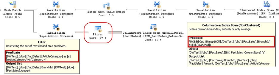
Figure 34-22. Execution plan for a query that uses a string attribute in the facts table to filter the article category
Obviously, in some cases, string attributes become part of the facts and should be stored in facts tables. However, in a large number of cases, you can add another dimensions table and replace the string value in the facts table with a synthetic, integer-based ID key that references a new table.
You already saw one such example of this with the ArticleCategory data. As another example, you may consider the situation when the facts table needs to specify the currency of a sale. Rather than storing a currency code (USD, EUR, GBP, and so forth) in a facts table, you can create a DimCurrency dimension table and reference it with a tinyint or smallint CurrencyID column. This approach can significantly improve the performance of queries against facts tables in Data Warehouse environments.
Summary
Columnstore indexes are an Enterprise Edition feature of SQL Server 2012-2014. In contrast to B-Tree indexes that store data on a per-row basis, columnstore indexes store unsorted and compressed data on a per-column basis.
Columnstore indexes are beneficial in Data Warehouse environments where typical queries perform a scan and aggregation of data from facts tables, selecting just a subset of table columns.
Columnstore indexes reduce the I/O load and memory usage during query execution. Only the columns that are referenced in a query are processed. Moreover, SQL Server introduces another batch-mode execution model that utilizes columnstore indexes. Rather than accessing data on a row-by-row basis, in batch-mode execution, SQL Server performs operations against a batch of rows, keeping them in fast CPU cache whenever possible. Batch-mode execution can significantly improve query performance and reduce query execution time.
There is a set of limitations in SQL Server associated with columnstore indexes. Some data types are not supported. Tables with nonclustered columnstore indexes become read-only. Fortunately, you can reference such tables in partitioned views, combining data from updateable tables with B-Tree indexes and read-only tables with nonclustered columnstore indexes. Moreover, tables with columnstore indexes support a partition switch, which allows you to add new data to a table by loading it into a staging table first and switching it as a partition to the main table afterwards.
Several factors improve the efficiency of Data Warehouse database systems. You should endeavor to reduce row and column sizes by using appropriate data types; avoid nullable columns; use CHECK and UNIQUE constraints when appropriate, and avoid using string columns in facts tables when possible.