
In a recording studio, what we hear (the effect that the environment or equipment has on the quality of sound we hear) is everything. What you are going to examine in this chapter is how to use room-measuring software to determine what anomalies exist in your control (listening) room and how effective your treatments are in achieving a good listening environment.
Let’s begin by understanding the reason I say “control (listening) room” and not a recording studio in general.
In a main tracking room, iso-booth, string room, etc., there is not a single specific (targeted) listening area. In those rooms there are multiple locations for microphone placement, depending on exactly what you may be recording.
In tracking rooms, you may be recording anything from amplifiers to vocals. Amps may have microphones placed in close proximity to them, perhaps a combination of microphones intended to pick up direct transmissions and room ambiance.
A vocalist may be a very tall adult or a small child. You may well be recording a saxophone or someone sitting down playing classical guitar. It will often be drums or entire bands.
In all of these cases, there are multiple locations within the rooms that microphones can and will be placed. The microphones in this case are the “ears” in the room. They “listen” and transmit what they “hear” to the recording chain. Although the rooms need to have a good sound, a lot can be accomplished even in fairly bad rooms through the combination of close micing instruments, amps, etc., coupled with gobos to provide at least a semblance of distance between instruments, which will minimize bleed from one instrument track into separate instrument tracks.
A control room, though, is a dedicated listening space. There is typically a fairly small “sweet spot,” which is the area that the person handling the engineering side of the recording (which may well include the mixdown of the music recorded) is going to be sitting in. This room needs to be treated in such a manner that the engineer can hear (in the listening position) an accurate representation of whatever is being recorded. Constructing and treating the room in order to obtain this “sweet spot” is the single largest goal in control room construction.
Due to the fact that there are acoustical issues that are psychoacoustic in nature, which means that the mind will interpret certain sounds to be something that they are not, testing a control room is an important part of the whole picture. Room anomalies might be able to trick the mind, but they cannot trick measuring instruments or software.
Everyone agrees on what good and bad sound quality is. In terms of loudspeakers, this has been proven with double blind listening tests performed by Floyd Toole[1] when he worked in Canada to determine relevant measurements for perceived loudspeaker quality. His work on this spanned a 20-year period beginning in the 1970s.
An important aspect of sound quality (especially in a critical listening environment) is that the equipment reproduces all sounds with the same amplitude at which they were recorded. This requires a frequency response from the equipment (amplifiers, mixing boards, speakers, etc.) capable of providing the same gain for all frequencies. If you have a setup that can achieve this, you should be able to produce a mix that translates in the real world without having to go back and forth between different systems outside of your room to verify the results.
An equally important aspect (to all of this) is the effect that the room has on the sounds transmitted into it. The best gear in the world won’t sound good in a room that makes it sound bad.
Subsequent research (by others) indicates that reflections from walls, ceilings, mixing boards, etc. can have effects that can negatively color the sound you hear while you mix, causing you to make poor or incorrect choices in EQ and reverb.
What we are going to examine here is how to test your room to make certain that there are no room anomalies affecting the music you are trying to mix.
The software we are going to examine here is RPlusD by Acousti Soft, Inc.[2] It is a very reasonably priced package with lots of bells and whistles. This software was developed under the Windows 2000 operating system and works within the XP, Vista, and Windows 7 operating systems.
It has also been run within Windows emulators on Mac machines. However, before purchasing it (to run on a Mac computer), you should download the demo program first (which is the full version, minus the key codes you need to turn on all the features) and test it to make certain it will run using your particular emulator.
There is also a freeware program called Room EQ Wizard that I have heard good things about but have never used. This software was written and tested under Windows XP and then subsequently tested with the Windows Vista operating system. It will also run on the Mac. (It has been tested on both the OS X 10.4 and 10.5 versions of the Macintosh operating systems; however, OS X 10.5 Leopard is the recommended operating system on the Macintosh.)
For the purposes of this book, we will only examine the RPlusD software. It would be much too involved to attempt to examine and compare different software packages, and it would make no sense whatsoever to examine professional stand-alone hardware designed for acoustic testing. Regardless of the software you eventually use, the concepts are the same.
There is an array of standard audio measurements, all of which are provided with RPlusD software. The basic measurement types, along with a brief description of the situation in which they are used, are described in the sections that follow. This chapter will explain the basic operation of audio analyzers, using examples from actual tests performed using RPlusD software.
The use, physical configuration, and external equipment required for use with RPlusD software will be explained. The chapter will conclude with a further explanation of the types of measurements with aspects of experimental procedures required to ensure accurate, precise, and repeatable results.
One great thing about this package is that the manufacturer is only a phone call away, answers his phone, and is right there to help you if you have any issues or questions. He has a Web site you can visit and also has a thread at Ethan Winer’s forum where he will directly answer any questions you might have (http://forums.musicplayer.com).
Let’s begin with an understanding of what exactly it is you need to measure (and treat) in order to make your room correct, and how you can go about determining this with the software.
Room anomalies are all of the various issues you read about in depth in Chapter 2, “Modes, Nodes, and Other Terms of Confusion.” These are issues like room modes, flutter echo, early reflections, etc. that will make it difficult, if not impossible, for you to just sit at your desk and mix a song that translates well in the real world.
An Energy-Time graph is shown in Figure 8.1. This result is used to compare direct sound levels emanating from the loudspeaker with reflection levels. Reflections originate from ceilings, walls, and floors when they are untreated.
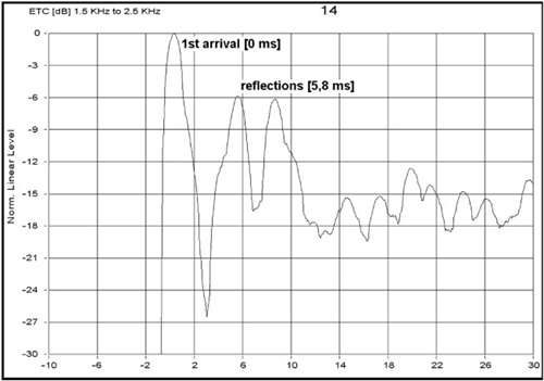
The mirror trick is a well-known way of determining offending surfaces. This is done as follows: One person sits in the listening area while a mirror is moved along a hard surface, such as a wall, by a second person. The observer looks at the mirror until the image of the loudspeaker appears. When this happens, the mirror is where the reflection occurs.
Measure from the loudspeaker to the surface at the mirror point. Then measure (from the mirror point) to the listener (the path length) and subtract the loudspeaker-to-listener distance (the direct source). The remaining distance can be converted to a time delay. Sound takes approximately 1ms to travel 1 foot. (If the measurement is in meters, sound takes about 2.91ms to travel a distance of 1 meter.) Multiply the distance difference by the appropriate time to obtain the time delay equivalent. Figure 8.1 is an example of a measurement that indicates direct sound and a subsequent reflection of that same sound. Note that the direct sound from the speaker occurs at t=0 seconds (reflections occur later).
Early reflections (also known as inter-stimulus delays (ISDs) and the Precedence Effect[3][4]) are known to create problems with the sound you will hear in a listening room. Early reflections are occurrences where the original signal from your speaker (lead location) combines with a reflected signal (lag location). There are three different phases of this effect:
Summing Localization (Phase I): This refers to reflections that combine with the original source before about 1ms.These reflections join the original signal with the reflected signal with the effect that a single sound appears to emanate from roughly halfway between the two sound sources. This has the added effect of modifying the original signal with a slight tonal coloring.
Localization Dominance (Phase II): This occurs roughly from 1ms to 10ms. The signals of the reflected and original sounds combine with the result being a stronger signal that is localized by the first signal source (which would be the monitor in the room, in this case).
Phase III ISDs: These are reflections that occur after about 10ms, and in this case, two distinct sources of the sound can be perceived, one near the lead and one near the lag.
Notice that the time span between signals is always an approximation. This is due to the fact that although everyone will experience the same results of these reflected effects on the lead sound source, not everyone will experience them in exactly the same time frames. For some people, a Phase I ISD may occur between 0ms and 2ms, etc. However, the above approximations appear (from the testing that has been performed to date) to be reasonably accurate in the majority of cases.
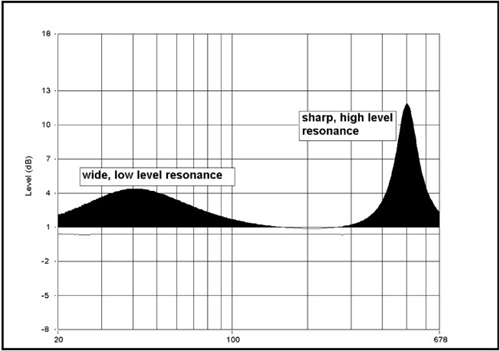
Resonant sounds are the consequence of the shape of the room and how the room dissipates sound energy, and they are the direct cause of peaks and dips in amplitude. Resonant sounds create a ringing effect and can be particularly bothersome, as well as more difficult to combat, than simple early reflections. Fortunately, these can be measured easily.
The degree of coloration due to a resonance is approximately proportional to the area under the curve as illustrated within the results of Figure 8.2, which is a comparison of two resonances that are roughly equal in audibility. You can see that the areas under the two different resonances are about the same, resulting in just about the same degree of coloration heard from each.
Resonances can be masked by other distortions, as well as program source material. Small resonances in the midrange are practically imperceptible when music is being played, but in voices and dialogue they are extremely audible. Resonances in the midrange are very troublesome to those monitoring voice recordings because our hearing is particularly acute when listening to speech. This is in the frequency range of 100Hz–5kHz (known as the “voice range”).
In each case, we can hear the distortions, which have the secondary affect of coloring the sound. We may not hear these particular distortions as distortions, and we cannot easily identify them just by listening. Sometimes, one type of distortion can sound very much like another. It is very difficult to determine the sources of coloration without taking measurements.
To determine the nature of distortions, as well as their likely causes, we can combine a little knowledge about sound with a few measurements and determine the cause. Then, armed with this information and the benefit of experience (or perhaps a good book), we can determine the best or most likely solution to the problem. Then the solution can be tested with another measurement. This is why computer-based audio analyzers are so widely used.
The problem with computer-based audio analyzers is twofold:
They are often used incorrectly and give erroneous results because of incorrect setup.
The setup and design of the measurement experiment itself is incorrect, leading to irrelevant or misunderstood results.
Sound is something that occurs in both a time realm and a frequency range. The two are intertwined. When we consider the response of a sound system (which in our case includes the room), we do so in terms of time or in terms of frequency. A frequency response and a time response are really the same thing, which is a mathematical representation of how a sound system responds to stimulus. One can be calculated from the other.
The impulse response is the fundamental measurement from which all other results are determined. It is best explained as follows: Imagine yourself checking the suspension of a car. You might jump on the bumper and watch how the car reacts. If the car bounces up and down numerous times, you know the shocks or springs need replacing. If this data could be recorded, it could be used to determine how the car suspension would respond to any bump in the road using a field of mathematics known as signal processing.
Similar to a car whose suspension needs new shocks, in signal processing language, the suspension is said to resonate. The shock absorbers critically damp the resonance by dissipating the energy that is normally cycled between kinetic and potential energy creating the resonance. It is absorbed and converted to heat in the shock absorber. The same action occurs in a sound-absorbing device. These devices are sometimes called dampers.
The chart in Figure 8.3 represents the raw data (from a room measurement) that is illustrating the actual response of the system. This result is processed to determine all other types of results, including the ETC curve in the impulse chart. Normally, the impulse response is converted to a frequency response.
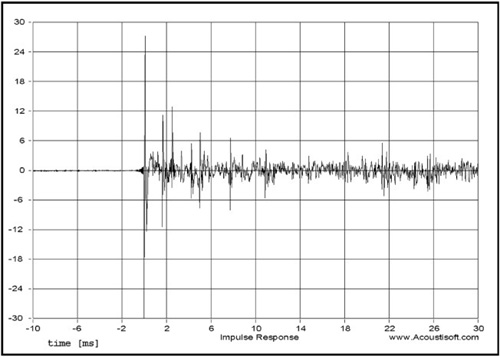
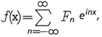
A frequency response curve is generated by applying a mathematical operation known as the Fourier Transform to an impulse response. A Fourier series is an expansion of a periodic function f(x) in terms of an infinite sum of sines and cosines. The Fourier series makes use of the orthogonality relationships of the sine and cosine functions. The computation and study of Fourier series is known as harmonic analysis and is extremely useful as a way to break up an arbitrary periodic function into a set of simple terms that can be plugged in, solved individually, and then recombined to obtain a solution to the original problem (or an approximation) to whatever accuracy is desired or practical.
The Fourier series, which is specific to periodic (or finite-domain) functions f(x) (with period 2π), represents these functions as a series of sinusoids, where Fn is the (complex) amplitude. Fourier theorized and later proved that any periodic sound (or non-periodic sound of limited duration) could be represented by Fourier analysis or created out of the sum of a set of pure tones with different frequencies, amplitudes, and phases, known as Fourier synthesis.
Fourier series
Now, having read the previous paragraphs, you’re probably thinking that a promise has been broken, that being the promise not to bury you in math. Nope, not true. I am not going to go any deeper into this than I already have. I explained this and gave you a peek at the beginnings of what is a rather lengthy series of mathematical equations just to show you how involved this really is and the lengths you would have to go to in order to work this out on your own. An in-depth study on the theories of acoustical analysis is really beyond the scope of this book, and it would violate the promise I made to you earlier.
I’m giving you just the very basics here, but am happy to say that the program can do all this for you. It can deliver all the information you need without you having to worry about any of the math.
Gating is sometimes used to erase many of the room reflections from the result before converting it to a frequency response. Figure 8.4 is an example utilizing gating. Notice the high degree of detail in this example. This is sometimes referred to as grass, and (as can be seen) when the frequency range increases, the problem increases.
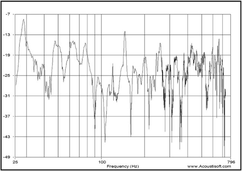
By problem, I mean this: Looking at this figure (beginning on the left), you can see that there are a series of very small jagged lines that break off from what could be viewed as the continuity of the main lines in the chart.
These are very small reflections (pieces of grass) that serve little purpose in analyzing the data. As you proceed from left to right, you can see that these become more and more obvious and annoying. Around 135Hz, centered from roughly -30dB to -32dB, there are no fewer than 12 of these small reflections. The higher in frequency, the greater the occurrence. By the time you reach around 600Hz, the grass is completely cluttering up the signal.
These small reflections are not only annoying, but they are also (in the long run) completely useless bits of information. They are so small in nature that by the time you finish dealing with the real issues (look at the huge peak and dip around 150Hz for one example), the grass will be gone.
The raw frequency response shown in the figure was directly calculated from an impulse response. It contains far too much detail to be useful. This problem is solved by reducing the applied gate to the impulse before this response is calculated or by using smoothing such as in the fractional octave response. A psychological response analysis uses a combination of these two methods (smoothing and gating) to provide a more accurate indicator of perceived spectral balance (if you can’t get your head around the perception of sound, please re-read the section on early reflections). However, a psychological response analysis is (computationally) much more intensive than a simple gated or fractional octave response. This really shouldn’t matter with the high-speed computers you are working with today. It (the psychological response) washes out detail, such as resonances, which are audible but do not affect the overall subjective frequency balance. Different methods of processing this raw data are useful for different purposes and will be explained in the sections that follow.
Many people like to use a waterfall response. This response mixes both time and frequency, and it looks very high tech as well as intuitive. The problem with waterfall displays is that they are not as intuitive as they look, and they generate confusion in terms of both time and frequency. They provide a distorted view of reality and are best ignored; however, they are in high demand so makers of analyzers must provide them. A serious user of audio analyzers with understanding would never use or even bother looking at a waterfall plot, except to see if noise is interfering with measurements or perhaps to witness “ringing” of lower frequencies.
The waterfall response is pretty, but can well be a wolf in sheep’s clothing. Changing the parameters changes the display, as can be seen in the figures that follow. There is no single correct set of parameters, making this measurement practically useless in real practice although powerful in visual effect. Compare Figure 8.5 with Figure 8.6, which is the same data reprocessed with different parameters.
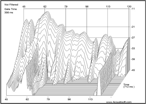
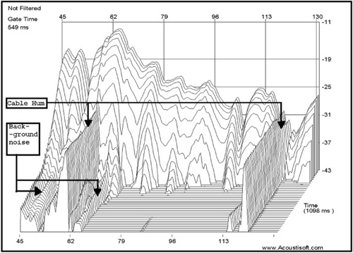
Notice the change in shape of the overall result. Which one is more correct? The answer is neither! Notice also that the extended portions along the time axis in the waterfall display always have a frequency response peak at the same frequency that is causing the resonance. The waterfall display dulls the resonance and, depending on settings, obfuscates the true nature of the response. The frequency response works best to quantify the nature of the resonance and is much more easily understood than the waterfall response. Its likely effect on what is actually heard is also much more evident because you can see the area affected by the resonance in the frequency response display, which gives a better indication of its overall audibility as well as a better indication of the exact offending frequency.
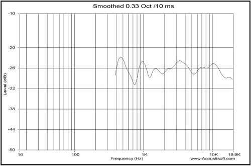
Human hearing operates over a very wide range, from approximately 20Hz to nearly 20,000Hz. This is a 1,000:1 difference in frequency, and it is difficult to show on a single graph. Fortunately, when interpreting a frequency response in terms of what is actually heard, this kind of detail is not necessary. The data can be smoothed using a moving average, or in lesser or older products using the less evolved method of forward and reversed IIR filtering of the data, which was the standard before high-speed/high-memory PC-based analyzers became prevalent. Smoothing data results in what is known as a fractional octave smoothed display. Coarse and smooth smoothing are shown in the two figures that follow. Figure 8.7 is an indicator of what to expect with coarse smoothing.
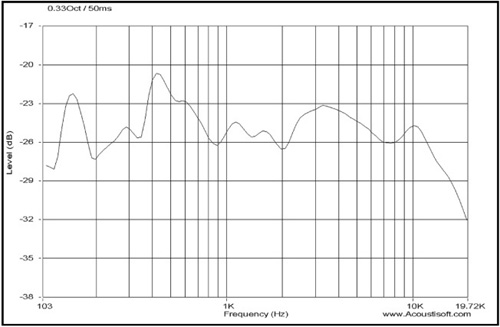
Figure 8.8 is an example of what you should expect to see with a smooth smoothing setting. Notice that the gate time is the same for both results. The reference “should expect to see” relates to the degree of detail displayed and not the actual frequencies. Your physical data will be different because it will be taken from a different room than the sample data.
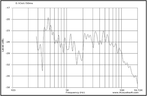
Notice that 1/10 octave smoothing presents a larger amount of detail than a 1/3 octave smoothing. Also notice that the minimum frequency is much higher while using the same gate time.
A tight resolution such as a 0.1 (1/10) or 0.05 (1/20) octave setting provides the level of detail needed to identify resonances. Whereas a 0.333 (1/3) octave setting is more indicative of overall frequency balance and can be useful for measuring room/speaker power response when enough measurements are taken to provide an accurate average.
Of these two methods used to “clean up” the frequency response, data smoothing (as pictured in the fractional octave results) is used for mid- and high-frequency responses. For room response, more detail is normally sought for the purpose of identifying room resonances. For this reason, you can simply gate the response to exclude the tail end of the impulse response (which eventually becomes just noise) and use the remaining data to calculate a raw unprocessed frequency response. See Figure 8.9 for an example of gating for this purpose.
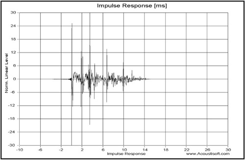
Notice the latter part of the impulse is not shown. This is the action of a gate. Gating (as applied to the impulse response) is meant to illustrate which data is included or excluded with a particular gate time, simply as a “visual aid” to see the nature of the type of gate used in this software (which is more suitable for audio than a conventional Gaussian[5] or Hanning[6] curve). The gate must be adjusted independently for the frequency response when viewing it. The gate here only shows what the gate is actually doing to the data for convenience.
Sometimes, a small gate time is used to exclude all or nearly all room reflections to get a more highly detailed view of the speaker response. This is normally done by knowledgeable users who truly understand the physical nature of systems in terms of mathematical descriptions. Most users would only use the fractional octave result. Fractional octave responses are also useful for fine-tuning and setting equalizers when doing final adjustments to correct for any small remaining acoustic anomalies.
The gate time (shown in Figure 8.10) is only 5.1 milliseconds (ms). Note that the lowest frequency shown in the response is 200Hz. Varying the gate time will change the lowest frequency that can be calculated.
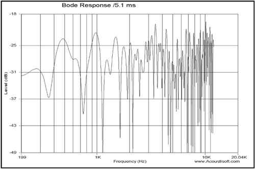
Notice that a 2ms gate time provides resolution down to 500Hz, while a gate time of 500ms provides resolution down to 2Hz. See Figure 8.11 to compare the readings in Figure 8.10 with the results of a longer gate time setting.
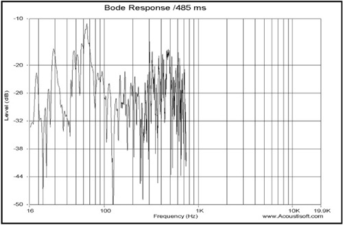
Longer gate times provide far too much detail at mid and high frequencies to be really useful. Notice the greater degree of detail associated in the longer gate time (485ms in this case). This is complex because a room response itself is highly complex. In fact, this high-frequency data is so complex that it really is useless to display it.
Gate time also affects the lowest frequency that can be shown in the fractional octave results, but a given gate time increases the lowest frequency that can be displayed while resolution is maintained. A 10ms gate time in the fractional octave measurement leads to a lower frequency limit of several hundred Hz rather than 100Hz, as is the case with unsmoothed data (see Figure 8.12). The data displayed is dependent on the resolution chosen while setting the gate time. Longer gate times are necessary with this measurement in order to see results at lower frequencies. Multiple averages tend to smooth out the effect of discrete reflections in the display while still showing their cumulative effect on response. This will be examined in greater depth later in this chapter.
Notice the lowest frequency that can be displayed with the 10ms gate using a resolution of 1/3 octave. Lower frequencies could be displayed, but the resolution would be less than 1/3 octave and therefore results would be misleading.
The psychological response (shown in Figure 8.13) is significantly more computationally intensive. It varies gate time with frequency (at low frequencies) as required to preserve its 3/4 octave resolution. At frequencies above 200Hz, the gate time is held at 5ms and fractional octave smoothing is applied at higher frequencies to smooth out data. This response is useful when multiple averages are not convenient, and it provides a full range response somewhat more indicative of the frequency balance heard by the listener than could be provided using a setting of 1/3 octave.
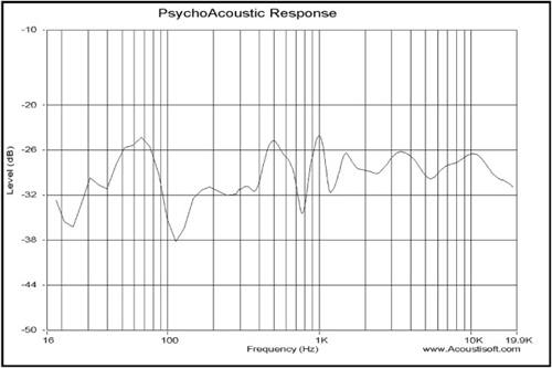
Notice that this is a very smooth, full-range response and that the effect of room reflections is removed with the gate time of 5ms at higher frequencies.
Learning how to set up and use room-testing software properly is critical if you expect the data you gather to be accurate. This is an area where you don’t want to rush. If you have gotten to the point where you are ready for room testing, you’ve already invested a lot of time, energy, and money in your project. Don’t throw that away just because it’s too much work to read the manuals (or watch the videos) in order to learn how to use the software properly.
People often rush into using an analyzer, thinking that they can get great measurements at a fraction of the cost. However, they often have little understanding of what the analyzer actually does. Often, big budgets and careful methods are thought to be frivolous and not worth the rates the practitioners charge. Nothing could be farther from the truth. Often, people who are inexperienced in the use of this type of software will end up producing results that only reflect incorrect wiring of the system. Because of this, they end up examining data that is meaningless due to their error. Other results may be generated from some experimental procedure they used that cannot provide measurements that reflect anything even remotely resembling reality, even though the measurements look perfectly valid. How the measurements are obtained is as (or perhaps even more) important than the actual results.
Measurements like those are often imprecise, irrelevant, and not repeatable. In earlier versions of the AcouistiSoft/ETF analyzers, it was not uncommon for Doug Plumb (the software engineer for both ETF and RPlusD, as well as the Owner of AcouistiSoft) to receive emails with questions about certain measurements that were taken by users of that software and recognize immediately that the measurement was meaningless garbage. Yet the user of the software never realized this. Changes to the software in RPlusD will largely prevent this from happening.
A typical measurement setup is shown in Figure 8.14.
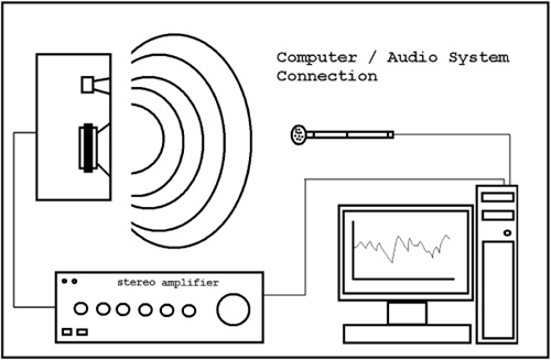
Notice that the computer software provides an excitation test signal for the audio system input, and that only one channel of information is provided. Only one channel should be measured at any one time because erroneous results occur due to interchannel interference when more than one speaker is playing the test signal during a measurement.
RPlusD is slightly more complex than other analyzers in its setup because it provides numerous checks to ensure that the measured results are relevant and not the result of unrelated phenomenon, such as an MP3 file playing music in the computer, an improperly connected sound card, if the sound card tone controls are not set properly, or even something as simple as a less than ideal sound card.
All of these can produce results that are less than precise, accurate, and repeatable. Care is required to ensure that measurements are both useful and relevant.
RPlusD software provides a system that gives a number of checks to ensure correct results. They are given in the next few sections.
The hardware setup to use this system may seem a bit daunting when you first get started, but it really is not as bad as it looks at first glance. If you have any problems getting started, please remember to pay careful attention to the details provided by Acousti-Soft in their various PDF files and the informative support videos they have on their Web site.
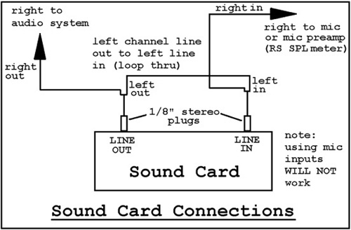
The loopback test is designed to verify that the sound card is operating correctly and to analyze sound that may be introduced via the sound card and computer system that it is connected to. Figure 8.15 is the connection required for performing a loopback test.
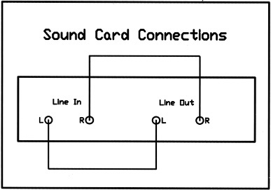
In addition, it is used to receive mic input and provide a signal to the system. This allows RPlusD to remove any frequency response anomalies that may be caused by the sound card itself or non-flat tone control settings. Tone controls may be set to provide a test signal that boosts certain frequencies that may otherwise be hidden with noise. It does make the software slightly more difficult to set up, but people having trouble with these connections likely are the ones that should have this additional verification. Neophyte users require more checks than those with experience and should play around with the analyzer and get comfortable with this checking of data before taking measurements they intend to rely on.
The typical wiring diagram for a sound card is shown in Figure 8.16. Many analyzers do not require the left-channel loopback connection, but it is a valuable addition to check the validity of data and sound card calibration, as well as provide the additional benefit of a very accurate mic/speaker distance measurement. (Notice the left-channel loopback connection for sound card calibration and mic-speaker distance referencing.)
Data gathering in RPlusD is a relatively easy process, but there are a few things you need to watch for. This program is relatively well laid out, but you still have to invest of yourself to make certain that the data you gather is accurate. As mentioned previously, this chapter will help you focus on the critical points, but it is ultimately up to you to see to it that this all works the way it is designed to. If you have problems with this, please remember that Acouisti-Soft is only a phone call (or email) away.
Figure 8.17 shows the indicators for the feature that estimates the mic-to-speaker distance. This provides a precise mic/speaker distance measurement that can be used to verify results for correctness. If the mic speaker distance isn’t correct, then something may be wrong and the measurements may not be correct. Sometimes the impulse needs to be shifted in the software to yield the correct results to get the first peak starting at 0ms. When the impulse is shifted to this position and the mic speaker distance is correct, the shifted measurement can be saved. The error was probably caused by an error in the auto-alignment system in RPlusD, which can never be perfect 100 percent of the time. In some cases, the manual input of mic/speaker distance is required, as in the case of sub-woofer-only measurements that do not provide enough high-frequency information for correct auto alignment to take place.
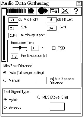
Sometimes, processing such as that which occurs in an EQ (or another processor) can give an additional delay in the signal, making the mic/speaker distance measure larger than it is in reality. This must be allowed for. It is impossible for a processor to make this distance appear shorter. This feature provides a valuable quick check to ensure the validity of the measurement.
Here are some items you need to pay attention to. In Figure 8.17, you can see the channel level indicators, signal-to-noise estimates, manual/auto mic speaker distance determination, Hybrid/Sweeps signal selection, and the special MLS test signal selection, (which is only used for electronic crossover emulation measurements of loudspeakers).
Pay attention to the values in the various data boxes; these are roughly the numbers that you should expect to see. If you see numbers that vary a great deal from these numbers (for example, positive numbers in the two boxes at the top of the screen), then there is something wrong with your setup.
The MLS test signal selection is only used for electronic crossover emulation measurements of loudspeakers. A discussion of this functionality is beyond the scope of this book and a different subject matter than what you are dealing with in this chapter. For further information on this topic, please visit the AcouistiSoft Web site.
The software provides indicators of an estimated signal-to-noise ratio as a piece of the data gathering process. The signal-to-noise ratio shown in Figure 8.17 is normally above 40dB for the loop-through (normally the left channel but this is switchable). Room measurements typically show around 25dB, but in many cases, a 15dB measurement is more than good enough. The test signal need only play at about 80–85dB to obtain these results. It is pointless to play the test signal any louder than what would interfere with normal conversations.
Playing the test signal too loudly may cause hearing damage or other health issues. It is easier to take large numbers of measurements when the test signal is played at a comfortable level. This also avoids user fatigue, which may (in and of itself) be the cause of a large number of erroneous results in data gathering. You can never have too many measurements for an average, but most people take far too few.
There are two different test signal types used with this software, Hybrid and Sweeps, as shown in the data gathering screen in Figure 8.17. Taking two consecutive measurements, one using the Hybrid signal, followed by one using the Sweeps signal is the best way to provide test measurements that will verify that the signals are not being affected by random background noise or distortion.
Comparing these two test signals will reveal the results of parasitic effects that would render the data (otherwise) useless.
Obtaining identical results when comparing these tests is a foolproof way of verifying that the data is unaffected by background noise, electrical noise, distortions in the system being tested, or noise in the room itself.
This preliminary procedure should always be used before running a full array of room measurements. RPlusD measures system gain, so an ideal setup will result in one measurement being directly overlaid with the second measurement, even though the sound-pressure levels of the two test signals will sound different.
It is not a problem adjusting your sound card output levels (if you want to raise or lower the volume during testing) because this will not affect the overall measurement of gain in the system.
During normal room testing, you will generally use the Hybrid signal, as it’s much more pleasant to listen to when performing a series of tests.
Figure 8.18 is a frequency graph of an estimate of the signal-to-noise ratio present in the measurement. Conventionally, a signal-to-noise ratio is a rating that describes a piece of equipment rather than a test result. In the case of this software, the estimated noise energy is calculated from the tail end of the impulse and compared with the measured impulse response in the form of a smoothed 1/3 octave frequency response.
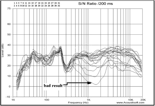
This response shows a much larger signal-to-noise ratio at low frequencies. The test signal is designed this way because frequency response at low frequencies tends to show a greater degree of variations and requires a higher signal-to-noise ratio so that test signal energy is much greater than noise. Also notice the erratic curve showing a bad result. (The curves and curve numbers are colored in the actual software package, which makes distinguishing them much easier than what you see here.) It’s a crude estimation, but it can make a single bad measurement obvious in a set (as identified in Figure 8.18). This measurement can be deleted before a subsequent average is performed.
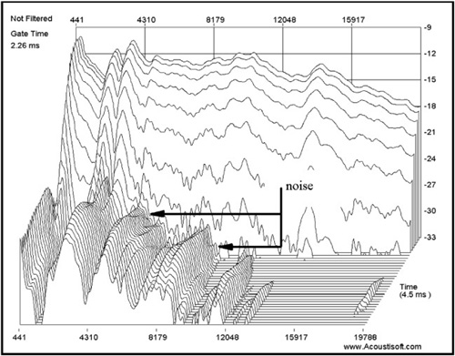
Although I do not find a lot of real value in the waterfall plot (Figure 8.19), it can indicate an approximation of the noise that may be affecting measurements in a similar way as the previous estimate. This is really the only useful result a waterfall plot can provide, and it is no more accurate than the display in Figure 8.18, but it is much prettier. (Notice the regions showing background noise—steady state and random.)
In order to use this (or any other) room software, you require sound card excitation, which means the connection of the sound card input to a microphone, as well as the connection of the output from the card to some external equipment. Your ultimate goal is (or if it is not it should be) to produce meaningful data that can be reproduced as desired.
In performing a measurement, the measurement itself must be repeatable and show the same result each time. A person using different equipment and slightly different microphone positions must be able to measure the same thing. The effect of the actual measurement mic location must be filtered out from results if an accurate representation of the system response is to be obtained because listeners never keep their heads in one position when listening to sound systems.
Single microphone measurements may be useful for finding certain system pathologies. For example, a resonance can be measured with a single mic measurement, but the measurement itself really only exposes the particular pathology rather than the response as a whole. Single mic measurements are useful for measuring the magnitude and time delay associated with reflections as well, but this too is a pathology of the system, not its response as a whole.
To measure the room response as a whole, multiple measurements must be taken. This normally consists of placing a mic at one location, taking a measurement, moving the microphone, and then taking another measurement. The correct number of averages must also be used to ensure that there are enough averages to ensure repeatability of the experiment for one who uses slightly different mic locations in the same setting.
Explanations of how to take good measurements are given in the next section with a diagram for each.
A single measurement for low-frequency response can show lots of parasitic effects from room reflections. Two measurements of low-frequency response with different mic positions are shown below. The differences are due to room reflections and these differences are highly dependent on microphone position (see Figures 8.20 and 8.21).
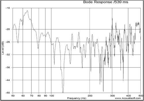
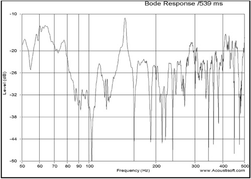
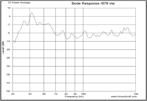
These random parasitic effects can be overcome by taking many measurements and averaging them. This makes resonances more obvious, which is what we want to measure when measuring the low-frequency response of rooms. The low-frequency response of rooms consists of nothing but a set of closely spaced resonances, which are, in fact, the transmission channels in a room (see Figure 8.22). Notice that the room resonances are much “stronger” and more apparent between 40Hz and 70Hz, with smaller issues above 70Hz.
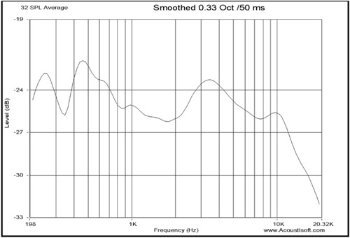
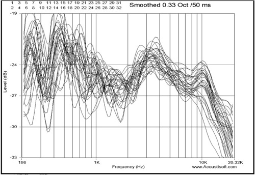
People often want to measure a room-speaker power response over the full audible range. This requires many measurements and combines the effect of the shape of the room along with the nature of the total loudspeaker response. Many mic locations are used. In this particular test case, there were 32 spread over a 2′ wide x 6′ long x 3′ high area (36 cubic feet).
In a small control room, an appropriate area may be something like a two-foot cube centered at the normal position of the mixing engineer. The spacing between the microphone positions determines the lowest frequency for which this measurement is repeatable. In this series of measurements, the microphone positions were more than one foot apart. The measurement is highly repeatable if the fractional octave smoothing is 1/3 (0.333) octave or lower for frequencies above a minimum wavelength of four times the mic spacing distance. The experimental result below is repeatable for the frequency range above about 250Hz; below 250Hz the results would be slightly different if the experiment were repeated with slightly different mic positions (see Figure 8.23). There is reduced sound power output in the mid-frequency range of this two-way loudspeaker. The speaker actually puts out less total power into the room at midrange frequencies due to the directional nature of the 6.5” woofer producing midrange frequencies. A three-way speaker would perform much better in this regard for that particular frequency region.
A single, or only a few, measurements would indicate a random nature in the data gathered. Due to this, no real conclusions would be able to be drawn. In Figure 8.24, you can see that the individual measurements are all markedly different, but they show a few things in common. Averaging the data filters out any of the random characteristics in the data, leaving us with the commonalities that exist within the various test positions.
If you only want to measure the loudspeaker response, take a lot of measurements (with random positions) near the axis of radiation of the speaker. The response can then be gated to eliminate most of the later room reflections. The few reflections remaining have a different effect for each mic location and will be averaged out. Figure 8.25 is an example of this type of data after averaging using the software.
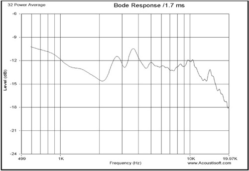
You can see the smooth response obtained by averaging multiple mic positions. Repeating this experiment with a new set of mic positions within the same area would yield very similar results.
Early reflections in a control room must be symmetrical and balanced; the RPlusD ETC system gives filtered bands that allow you to see reflected sounds originating from the independent drivers in a loudspeaker system (see Figure 8.26).
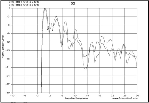
Notice the first reflection from the tweeter is higher than from the midrange. A slight reorientation of the loudspeaker may be all that is required to fix this. This measurement is also useful for testing symmetry in reflections between the left and right channel.
Let’s take a moment here and discuss (again) the symmetry of the control room and this particular test.
When performing this test for the purpose of measuring the acoustical symmetry in a room, my personal recommendation would be for you to use a painstakingly methodical approach, using (first) the same speaker and channel for both sides of the room. The reason I say this is because unless you are using some of the best paired speakers around, speakers will often have differences between them. The same is true for the gear you may be using.
Once that signal leaves the computer, even if you split the signal into a mono pair, the entire signal path through your gear and speakers might well produce totally different results left to right. Thus, setting up both speakers (in a symmetrical layout) in a room that is acoustically “perfect” does not necessarily guarantee that testing will indicate room symmetry.
However, for the purposes of this test, if you use the same signal path, meaning the same speaker and system chain, you know that the signal you receive at the microphone is identical side to side (at least from the perspective of the initial signal from the equipment). Then if any anomalies crop up, it is the room that makes the difference, not the equipment. If you are using new speakers and a system that you feel is spot on, then you could well skip this special test. However if something strange seems to crop up, this is always a good test to verify that it is indeed the room that is at fault and not the gear.
Once that is completed, it would make a lot of sense to test the left and right channels fully to verify if the speakers and signal chain are in fact exactly the same. Making minute adjustments then to the EQ of one channel would make it possible for you to fully balance your system. For those of you using state-of-the-art, top-of-the-line gear, this should not be an issue.
You probably have gone to great lengths and a lot of expense to try to do this right. From isolated assemblies to room treatments, doing it right is neither inexpensive nor necessarily easy.
Knowing what you achieved in the end (from the perspective of isolation) is probably as important to you as the final room finishes. Testing your room-to-room isolation before installing all of your finishes would make a lot of sense. It’s not that difficult to add some layers of drywall before a space is finished, but making a difference after the room is completed would be a huge expense.
Isolation testing is another area where this software shines.
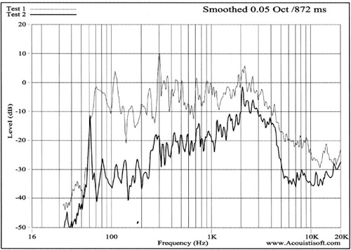
RPlusD is easily used to measure the effectiveness of sound isolation schemes. The procedure involves taking sound-pressure level measurements, with the door to the room being tested in both the closed and open position. This will measure the effectiveness of whatever weather stripping you installed for the door along with the TL values for the wall/door assembly as a whole. Figure 8.27 shows the SPL responses for a typical room taken with the door in both open and closed positions.
Note that in this particular test, it’s important to use the manual speaker-mic distance in the software to compare the two, and it is equally important that the dimension entered into the software to identify the microphone location is very accurate.
In some cases, wooden doors will act like windows over some narrow frequency ranges, and well-insulated heavy doors will show a uniform decrease in sound level that is perhaps a 20–30dB reduction or even more.
In the particular case above, the test was done using a standard hollow-core door assembly. Test 1 was performed with the door in the open position. Note that the door resonant frequency, as well as the area of coincidence, can clearly be seen in this comparison. The resonant frequency is that spot at just about 62Hz where there is no isolation (the two frequencies join). Coincidence in this door is in the frequency range of 2kHz to roughly 4.5kHz. Notice how little isolation there is in that range. Adding mass, damping, and weatherstripping to this door would definitely help you go a long way toward helping to isolate this space.
You can clearly use this feature to help you assess your success (perhaps further needs) when it comes to isolation.
RPlusD also provides a full emulation of the Behringer FBQ 2496 parametric equalizer. The filters in the software duplicate the settings in the equalizer, and the filters are run through the data in the time domain rather than the EQ curve being added as a delta curve as in other software. RPlusD does not require a measure-EQ-measure-EQ cycle. You measure once, determine your EQ setting in the software, and then apply it to the EQ only once. Precision EQ for midband response is highly beneficial. Problematic room modes are normally best treated with absorbers, but when EQ is the only choice, then RPlusD combined with a Behringer EQ is a very powerful tool, due to the nature of RPlusD and the fine adjustments available of the Behringer unit (see Figure 8.28).
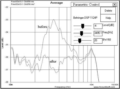
Notice that the software provides the effect of the EQ on any measurement in real time as you adjust the EQ controls in the software while looking at the measurement. RPlusD does not emulate the anti-alias filter in the Behringer unit. Its gentle decline is best compensated for by a single-filter 1dB boost at 20KHz using a 3-octave (180/60) bandwidth setting.
Just a few notes here about parametric EQ and DSP (Digital Signal Processing).
Although the documentation for this software uses a Behringer unit as its example, the crossover filters themselves are universal, meaning that any DSP EQ will behave the same way provided it uses the “Standard Bilinear Transform,” which it should for mapping frequencies in and out of the digital domain. This is never mentioned in spec sheets and is always used. There is no reason for a designer of a DSP EQ system to use any other mapping method.
Digital signal processing has come a long way from the time when it started, but it is still not a substitute for a well-designed, well-treated room. However, within a well-treated, well-designed room, it can go a long way toward helping you tweak out that last little bit that makes the difference between an average room and a really good room. (Really great rooms can stand on their own merit.)
So please don’t let yourself get sloppy because you think that when all is said and done you can deal with anything remaining by simply using DSP—it just isn’t going to happen.