
5 Theoretical Predictions of Electro-Optic (EO) Effects in Polymer Wires
One of the important applications of molecular layer deposition (MLD) is nonlinear optical polymers that are the key materials for photonic devices such as light modulators, optical switches, tunable filters, wavelength converters, and so on.
In the present chapter, nonlinear optical effects, especially EO effects in polymer wires with designated molecular sequences, are predicted theoretically [1, 2 and 3].
5.1 Molecular Orbital Method
In order to design EO polymer wires, the molecular orbital (MO) method is used. In the present section, the MO method is briefly reviewed.
Figure 5.1 shows models for Hamiltonian in the MO calculations. In this example, the system consists of N electrons. The Hamiltonian of the whole system is written as follows.
Here, i(i = 1,2, … , N) and j(j = 1,2, … , N) represent ith electron and jth electron, respectively. qi is the position of the ith electron, qj is the position of the jth electron, Δi is the Laplacian for the ith electron, V(qi) is the interaction energy between the ith electron and nuclei, m is the mass of an electron, and e is the charge of an electron. The second term represents interaction energy arising from the Coulomb force between electrons.
A one-electron Hamiltonian for the ith electron is expressed as follows:
Here, ϕj(qj) is the wavefunction of the jth electron. ϕj(qj) is called the molecular orbital. The second term represents the interaction energy between the ith electron and the jth electron, where the jth electron is regarded as an electron cloud. The interaction energy is calculated as an expected value determined by using the charge density distribution of the jth electron, eϕj*(qj) ϕj (qj).
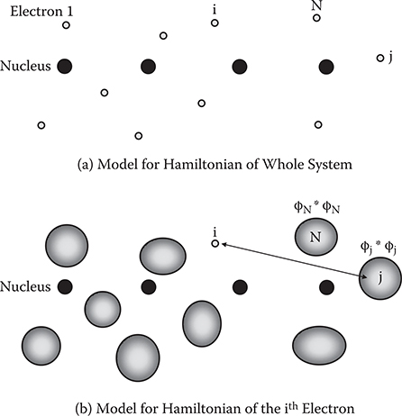
FIGURE 5.1 Models for Hamiltonian in the molecular orbital calculations.
Schrödinger equations for the whole system Hamiltonian and the one-electron Hamiltonian are respectively given as follows:
Here, Ψ is a wavefunction of the whole system.
The molecular orbitals can be expressed as linear combinations of wavefunctions in atoms (atomic orbitals) χr.
An example of the relationship between ϕi and χr is schematically shown in Figure 5.2 for a case of C2H2. ϕi is built up by χr with amplitude of cir. cirs are determined by the variation principle, namely, by finding a set of cirs that minimize εi in the following formula.
The minimized εi gives the energy eigen value for the molecular orbital of ϕi = ΣrCirχr. In a system with N electrons, N molecular orbitals are derived. However, in real systems, two spin states (α, β) are involved for one molecular orbital, resulting in 2N molecular orbitals. So, we should renumber the molecular orbitals including spin states as ϕi(i = 1,2,…,2N).
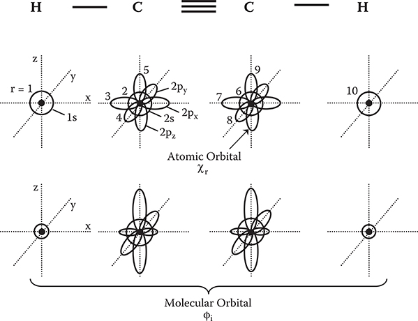
FIGURE 5.2 Schematic illustration of the relationship between atomic orbitals and molecular orbitals.
Figure 5.3 shows schematic illustrations for energy levels of molecular orbitals and electron occupation in many-electron wavefunctions built up from the molecular orbitals. The many-electron wavefunctions represent the actual electronic state of the whole system. The wavefunction for the ground state is expressed as follows,
where, is a permutation operator and p is the number of permutations. Electrons occupy molecular orbitals ϕ1, ϕ2,..., and ϕN.
In the 0th approximation, many-electron wavefunctions for the excited states are written as follows
where, i→j represents that an excited state, where an electron is excited from ϕi to ϕj. Φi→j is called the configuration function.
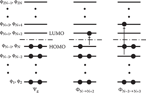
FIGURE 5.3 Schematic illustrations for energy levels of molecular orbitals and electron occupation in many-electron wavefunctions built up from the molecular orbitals.
In order to improve the accuracy of the molecular orbitals obtained previously, the variation principle is again applied to the following equation.
Then, a set of improved cirs that minimize E are obtained. The minimized E gives the ground state energy Eg for Ψg.
In general, the excited states are expressed as linear combinations of Φi→j as follows.
Cn, i→j s are determined by the variation principle, namely, by finding a set of Cn, i→j s that minimize En in the following formula.
The minimized En gives the energy eigen values for the excited states of Ψn = Σi,jCn,i→jΦi→j.
Thus, wavefunctions and energy eigen states are obtained.
5.2 Nonlinear Optical Effects
Nonlinear optical phenomena can be understood using the spring analogy shown in Figure 5.4. In a spring, displacement x is proportional to external force F for small F. With increasing F, the spring stretches rapidly with a nonlinear relationship between x and F. Nonlinear optical phenomena can be similarly described by replacing x with polarization P and F with electric field E as follows.
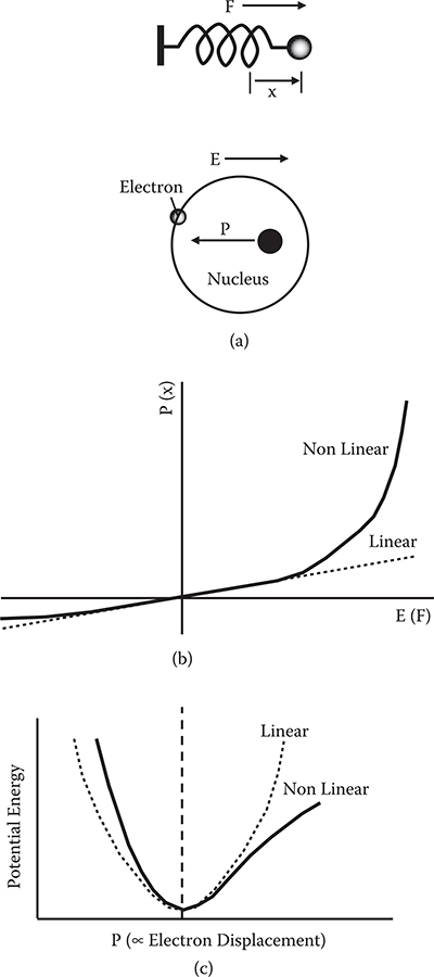
FIGURE 5.4 Model for the nonlinear optical phenomena using the spring analogy.
Here, ε0 is the dielectric constant in vacuum, χ(1) is linear susceptibility, and χ(2) and χ(3) are nonlinear susceptibilities. When E is small, P is proportional to E.
With increasing E, the contribution of the E2 or E3 term becomes dominant. The E2 and E3 terms induce second-order and third-order nonlinear optical effects, respectively.
E can be expressed by a sum of electric fields of light with an angular frequency of ω, Eopt = Ee–jωt, and an externally applied electric field, EDC, as follows:
The term E2 gives Eopt2,EDC,Eopt,EDC2 which are origins of the second-order nonlinear optical effects, and the term E3 gives Eopt3,Eopt2,EDC,EoptEDC2,EDC3 which are origins of the third-order nonlinear optical effects. When we focus on the term Eopt2, Equation (5.12) can be written as
Polarization oscillating at 2ω generates light with angular frequency of 2ω, that is, the second harmonic generation (SHG) arises. When we focus on the term Eopt3, Equation (5.12) can be written as
Polarization contains a 3ω component, generating light with angular frequency of 3ω, that is, the third harmonic generation (THG) arises.
When we focus on the term EDCEopt, Equation (5.12) can be written as
Since the refractive index, n, is a function of ε0χ(1) + ε0χ(2) EDC, n can be expressed as follows.
Considering the relationship of ε0χ(1) ≫ ε0χ(2) EDC, n is rewritten using a Taylor expansion as
By putting n0 = f(ε0χ(1)) and r ∝ f′(ε0χ(1))ε0χ(2)
is obtained. This formula implies that the refractive index changes linearly with an applied electric field, which is the Pockels effect. r is the Pockels coefficient.
When we focus on the term EDC2Eopt, Equation (5.12) can be written as
As in the Pockels effect,
is derived. This implies that the refractive index changes in proportion with E2, which is the Kerr effect. R is the Kerr coefficient. The Pockels effect and the Kerr effect are used for various kinds of EO devices such as light modulators, optical switches, tunable filters, and so on.
The relationship between E and P can be translated into the electronic potential energy vs. polarization curve as Figures 5.4(b) and (c) show. When E and P are linearly related, the potential energy curve is parabolic. This corresponds to the fact that the potential energy of a spring is proportional to x2. When nonlinear terms predominate, the potential energy curve deviates from the parabola.
In Figure 5.5, various kinds of nonlinear optical effects are drawn visually. SHG can be understood by the illustration shown in Figure 5.5(a). Due to the term E2 in Equation (5.12), the potential energy vs. polarization curve becomes asymmetric. Therefore, when light with angular frequency of ω is introduced, asymmetric responses of P are induced, resulting in a P component with 2ω. The P oscillating at 2ω emits light with angular frequency of 2ω. For THG, due to the term E3 in Equation (5.12), the potential energy vs. polarization curve deviates from the parabola symmetrically as shown in Figure 5.5(b). Then, when light with an angular frequency of ω is introduced, the P component with 3ω is induced, emitting light with an angular frequency of 3ω.
For the Pockels effect, in which the refractive index changes linearly with an applied electric field EDC, the potential energy vs. polarization curve deviates from the parabola asymmetrically as shown in Figure 5.5(c). When light is introduced, in the model shown in Figure 5.5(c), a larger P disturbance, ΔP, is induced for EDC > 0 than for EDC < 0 since the slope of the curve is smaller for EDC > 0 than for EDC < 0. Large ΔP tends to give rise to a large refractive index. Thus, with an increase of the applied electric field, the refractive index increases.
Measures of second-order and third-order optical nonlinearities for a molecule are respectively given by molecular second-order and third-order nonlinear susceptibilities β and γ. For aggregates of many molecules, macroscopic measures of second-order and third-order optical nonlinearities can be given by χ(2) originating from βs and χ(3) originating from γs. EO coefficient r, which is proportional to χ(2), is used as the measure for the Pockels effect.
In general, the potential curve deviation becomes large in highly polarizable systems. Figure 5.6 schematically illustrates electron-cloud polarizations induced by an electric field. In dielectric materials such as lithium niobate (LN), electronic polarization is not large because electrons are localized near atoms, regarded as a strong spring. In semiconductors, electron clouds are widely spread, regarded as a weak spring. Therefore, compared to dielectric materials, large electronic polarization is attainable in semiconductors. Organic materials, especially polymers with long conjugated wires, have electrons delocalized one dimensionally, that is, they are regarded as natural quantum wires. The one-dimensional characteristics are favorable for efficient electronic polarization induced by an electric field in the wire direction. This is why organic materials seem promising for nonlinear optical devices.

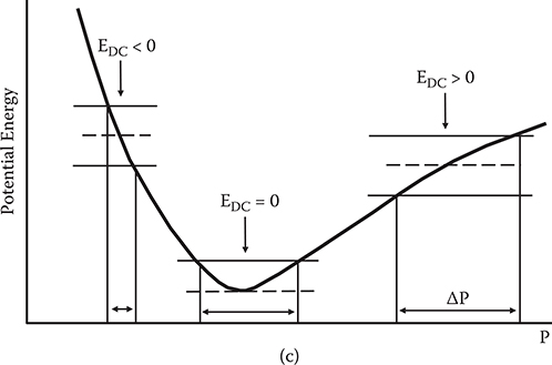
FIGURE 5.5 Visual explanation for (a) second harmonic generation, (b) third harmonic generation, and (c) the Pockels effect.
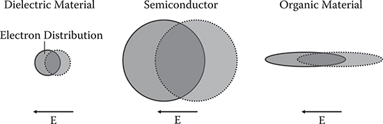
FIGURE 5.6 The reason why organic materials are promising.
5.3 Procedure for Evaluation of the eo Effects by the Molecular Orbital Method
Molecular second-order nonlinear susceptibility, or hyperpolarizability in the wire direction, is shown in Equation (5.22) based on Ward’s expression [4,5]
for the Pockels effect, and
for SHG.
In Equations (5.22) and (5.23), rgn is the transition dipole moment between the ground and excited states and rn’n is that between two excited states. Δrn is the difference in the dipole moment between the excited and ground states. ħωng is the excitation energy from the ground state to the excited state. ħω is the energy of incident photons.
rgn, rn’n, and Δrn are expressed by the following equations,
where, Ψg is the wavefunction of the ground state and Ψn is the wavefunction of the excited state. These wavefunctions are expressed by Equations (5.7) and (5.10), and are constructed by molecular orbitals ϕi. Then, rgn, rn’n, and Δrn are expressed as follows [5].
Here, the primed summations indicate to exclude terms, in which i = k and j = l simultaneously. rgn, rn’n, and Δrn can be calculated from Equations (5.27) through (5.30) once a set of molecular orbitals are obtained by the MO method. Using the rgn, rn’n, and Δrn, β can be calculated from Equations (5.22) and (5.23).
In the present simulation [1–3], the Austin Model 1 (AM1) method, a semi-empirical molecular orbital method was used for calculations of molecular orbitals. AM1 was developed by modifying the core repulsion function in the modified neglect of the diatomic overlap (MNDO) method. Using these molecular orbitals, the ground state wavefunction Ψg, a product of the occupied orbitals, and configuration functions, Φi→j, a product of the orbitals with one-electron excitation from occupied orbital ϕi to unoccupied orbital ϕj were made. Excited states Ψn, expressed by linear combinations of configuration functions as Equation (5.10), were determined by single-excitation configuration interaction (CIS). CI calculation involved eight unoccupied orbitals above the lowest unoccupied molecular orbital (LUMO) and six occupied orbitals below the highest occupied molecular orbital (HOMO). 2-methyl-4-nitroaniline (MNA) was used as the standard molecule. From the calculation, β of 13 × 10−30 esu for SHG with a fundamental wavelength of 1.06 µm was obtained. This agrees fairly well with the 12 × 10−30 esu reported by Garito et al. [6].
5.4 Qualitative Guidelines for Improving Optical Nonlinearities
Figure 5.7 shows the microscopic origins of second-order and third-order optical nonlinearities. As mentioned in Section 5.2, the potential energy curve in linear systems is parabolic. In nonlinear systems, however, it is not. This potential curve deviation from the parabola induces a variety of nonlinear phenomena. Second-order optical nonlinearity arises from the asymmetric potential curve deviation (see Figure 5.7(a)). Third-order optical nonlinearity arises from the symmetric potential curve deviation (see Figure 5.7(b)). The larger the potential curve deviation becomes, the larger the induced nonlinear optical effect becomes.
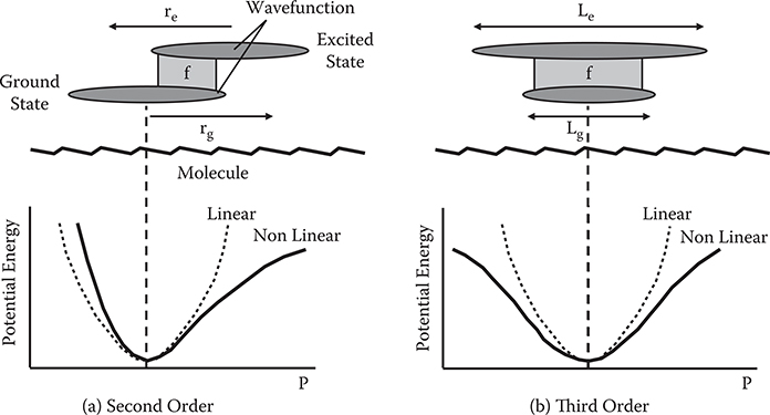
FIGURE 5.7 Microscopic origins for (a) second-order and (b) third-order optical nonlinearities.
The driving force for this potential curve deformation is explained in terms of the shape of the wavefunction as shown in Figures 5.7(a) and (b). Consider the ground state g and one excited state e, that is, a two-level model, for simplicity. When perturbation is induced in a molecule by incident light or electric field, mixing of the excited state wavefunction into the ground state wavefunction occurs, deforming the potential curve. Therefore, the first approach to improving optical nonlinearity lies in promoting the mixing rate of ground and excited states, that is, promoting the oscillator strength, f, between the ground and excited states. Here, f ∝ rge2, which can be increased by promoting the wavefunction overlap between the ground and excited states.
However, increasing only the wavefunction mixing rate is not in itself sufficient to increase the potential curve deformation. For example, when the ground and excited state wavefunctions have a similar shape, mixing the wavefunctions results in only a small change in electron distribution. Consequently, there is only a small potential curve deformation. Thus, another approach to improving optical nonlinearity is promoting the wavefunction difference between the ground and excited states. From the arguments mentioned above, the qualitative guidelines described in subsections 5.4.1 and 5.4.2 are derived.
5.4.1 FOR SECOND-ORDER OPTICAL NONLINEARITY
Promote wavefunction overlap between the ground and excited states, increasing oscillator strength f ∝ rge2.
Promote wavefunction separation between the ground and excited states, increasing the dipole moment difference Δr = re − rg. Here and .
Consequently, second-order optical nonlinearity is proportional to the product of f and Δr, that is,
The result is consistent with the two-level model expression for molecular second-order nonlinear susceptibility in Equation (5.22),
5.4.2 FOR THIRD-ORDER OPTICAL NONLINEARITY
Promote wavefunction overlap between the ground and excited states, increasing the oscillator strength f ∝ rge2.
Promote differences in the spread of wavefunctions between the ground and excited states, increasing ΔL=Le-Lg. Here Le = ∫ Ψe*r2Ψed3x = (r2)e and Lg = ∫ Ψg*r2Ψgd3x = (r2)g are measures of wavefunction spread.
Consequently, third-order optical nonlinearity is proportional to the product of f and ΔL, that is,
For both second-order and third-order optical nonlinearity, note that rge2 and re−rg, or rge2 and (r2)e−(r2)g are not independent, but are in a trade-off relationship. Therefore, it is concluded that the balance of the wavefunction overlap and wavefunction separation, or the balance of the wavefunction overlap and wavefunction spread difference, must be considered in optimizing nonlinear optical effects.
5.5 Enhancement of Second-Order Optical Nonlinearity by Controlling Wavefunctions
The effect of wavefunction shapes of the excited state (n) and the ground state (g) on rgn , Δr= rn−rg, and β is schematically illustrated in Figure 5.8. From left to right, wavefunction separation between the excited and the ground states increases while wavefunction overlap between the two states decreases, that is, Δr increases and rgn decreases in a trade-off relationship. According to Equation (5.31), in the two-level model, β is expressed by β ∝ rgn2 Δr . So, β becomes the maximum in the middle wavefunction shape. Both the wavefunction separation and wavefunction overlap must simultaneously be considered to optimize β.
Furthermore, as described in Section 5.5.2, Δr and rgn depend on the dimensionality of the conjugated systems. Therefore, it is concluded that β is expected to have its maximum in a wavefunction shape of intermediate wavefunction separation with an appropriate conjugated system dimensionality existing somewhere between zero and one, that is, between the quantum dot condition and the quantum wire condition.
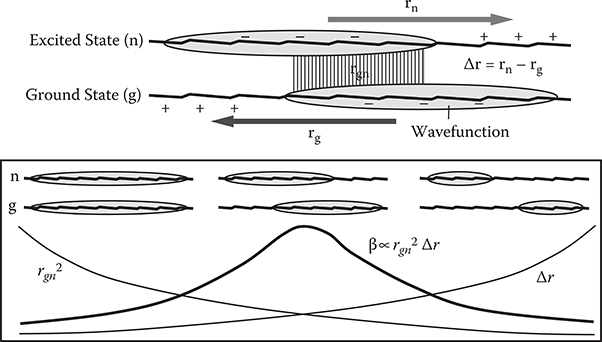
FIGURE 5.8 Effect of wavefunction shapes on rgn, Δr, and β. From T. Yoshimura, “Enhancing second-order nonlinear optical properties by controlling the wave function in one-dimensional conjugated molecules,” Phys. Rev. B40, 6292–6298 (1989).
5.5.1 EFFECTS OF WAVEFUNCTION SHAPES
In order to examine different wavefunction shapes, four types of conjugated polymer wires shown in Figure 5.9 were considered. The wires have backbones of polydiacetylene (PDA) structures and substituted donor (D) and acceptor (A) groups. DA, DAAD, DADA, and DDAA show the types of donor and acceptor substitution, and the numbers following them are the number of carbon sites (Nc) in the wire. As Figure 5.10 shows, the donor and the acceptor have a tendency to push electrons away and pull electrons closer, respectively, when electrons are excited. So, wavefunction shapes can be optimized by adjusting donor/acceptor substitution sites in the wires using push and pull effects as well as by adjusting wire lengths. In the present model, the donor is NH2 and the acceptor is NO2. β was calculated by varying Nc from 10 to 34.
Figure 5.11 shows molecular orbitals near the Fermi surface for DA34, DAAD34, DADA34, and DDAA30. Here, GM (M = 1, 2, 3) denotes the occupied molecular orbitals and EN (N = 1, 2, 3) unoccupied molecular orbitals. Gl is HOMO and El is LUMO. In DA34, DAAD34, and DADA34, the charge separation in the wire direction appears mainly in the HOMO and LUMO. In other molecular orbitals, electrons in the wires tend to be delocalized. In DDAA30, however, considerable charge separation appears in E2 and E3 orbitals as in LUMO.
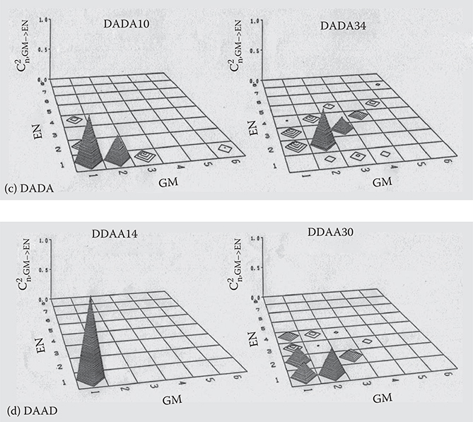
Figure 5.12 shows C2n, GM→EN as a function of GM (M = 1,2,. .., 6) and EN (N = 1,2, ..., 8) for the first excited states (n = 1) in DA10, DA34, DAAD10, DAAD34, DADA10, DADA34, DDAA14, and DDAA30. C2n, GM→EN is the fraction of the configuration function Φi j ® involved in Equation (5.10). The height of the pyramid indicates C2n,GM→EN. For the short polymer wires with Nc = 10 or 14, the first excited states consist mainly of the configuration functions with small GM and EN, which means that the configuration interaction can be calculated sufficiently using only a few occupied and unoccupied molecular orbitals. For the long polymer wires with Nc = 30 or 34, the pyramids are distributed more widely than for the short molecules. The heights of the pyramids tend to decrease rapidly with increasing GM and EN. This suggests that six occupied orbitals and eight unoccupied orbitals are enough to calculate the configuration interaction for the polymer wires shown in Figure 5.9.
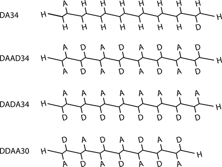
FIGURE 5.9 Four types of conjugated polymer wires with polydiacetylene backbones. From T. Yoshimura, “Enhancing second-order nonlinear optical properties by controlling the wave function in one-dimensional conjugated molecules,” Phys. Rev. B40, 6292–6298 (1989).
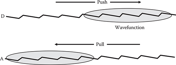
FIGURE 5.10 Push–pull effects on wavefunction induced by donor–acceptor groups.
Combining these results of C2n, GM→EN shown in Figure 5.12 with the shape of the molecular orbitals shown in Figure 5.11, the wavefunction shapes are clarified. Figure 5.13 shows structures and schematic wavefunction shapes for DA34, DAAD34, and DDAA30. In DA34, the Gl -> El component, corresponding to the HOMO-to-LUMO transition, is extremely small. The wavefunction separation then becomes small, which corresponds to the wavefunction condition on the left side in Figure 5.8. In DAAD34, finite Gl -> EN and GM -> El components appear, resulting in a considerable wavefunction separation, which corresponds to the condition in the center in Figure 5.8. In DDAA30, Gl -> EN components predominate, and furthermore, the EN orbitals exhibit considerable charge separation, inducing the large wavefunction separation like on the right in Figure 5.8. Thus, it is found that wave-function separations increase in the order of DA34, DAAD34, and DDAA30.
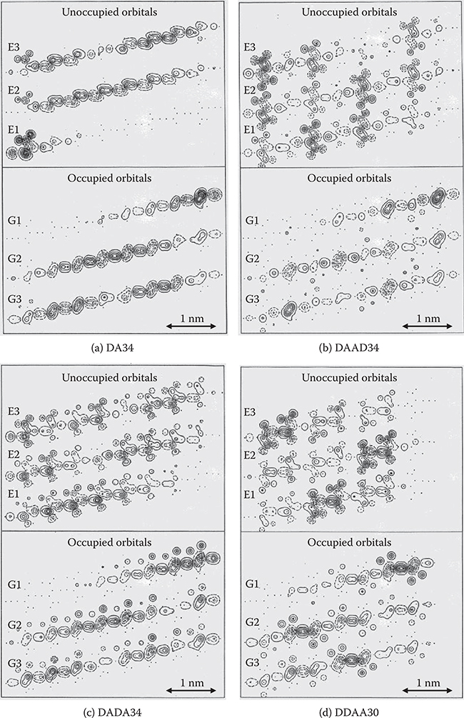
FIGURE 5.11 Contour diagrams of molecular orbitals near the Fermi surface in plane z = 0.06 nm for (a) DA34, (b) DAAD34, (c) DADA34, and (d) DDAA30. From T. Yoshimura, “Enhancing second-order nonlinear optical properties by controlling the wave function in one-dimensional conjugated molecules,” Phys. Rev. B40, 6292–6298 (1989).
Figure 5.14 shows the calculated molecular second-order nonlinear susceptibility for DA34, DAAD34, DADA34, and DDAA30 at a detuning energy of 0.2 eV from the first excited states. Here, ρβ represents β normalized by molecular wire lengths. Although calculations were carried out by using Equation (5.22) involving 48 excited states, the major contribution to ρβ was from the first excited state. Thus, the overall tendencies in Figure 5.14 can be explained in terms of the wavefunction of the first excited state. Δr increases and rgn decreases in the order of DA34, DAAD34, DADA34, and DDAA30. Consequently, ρβ becomes small in DA34 and DDAA30, and becomes largest between them, in DAAD34, which exhibits a medium wavefunction separation. This parallels the tendency of the qualitative guideline shown in Figure 5.8 and indicates that a balance between rgn and Δr is important to improve β.
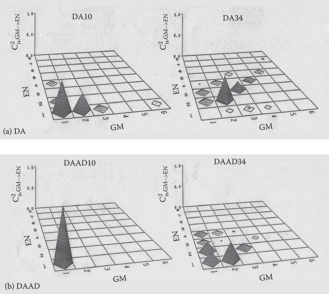
FIGURE 5.12 C2n, GM→EN for the first excited states in (a) DA, (b) DAAD, (c) DADA, and (d) DDAA. From T. Yoshimura, “Enhancing second-order nonlinear optical properties by controlling the wave function in one-dimensional conjugated molecules,” Phys. Rev. B40, 6292–6298 (1989).
5.5.2 EFFECTS OF CONJUGATED WIRE LENGTHS
Morley reported that molecular second-order nonlinear susceptibility increases with the chain length in polyenes with donor–acceptor substitution at the chain ends [7]. It is expected from the result that the PDA wires substituted by the donor–acceptor exhibit wire-length dependence of optical nonlinearity. In Figure 5.15, calculated ρβ is plotted for DA, DAAD, DADA, and DDAA as a function of Nc, which corresponds to the wire length. Nc dependence of ρβ is greatly affected by the donor–acceptor distribution. In DA and DAAD, ρβ is maximized at Nc = 18, which corresponds to a wire length of ~2.2 nm, and in DDAA, at Nc = 22. Morley reported similar behavior in β versus Nc curves in polyenes and polyphenyls having one donor and one acceptor at opposite sides [7]. In DADA, ρβ increases with Nc in a range of 10 ≤ Nc ≤ 34.
ρβ is smallest in DDAA. DAAD has the largest ρβ of about 3000 × 10−30 esu/nm at Nc = 18. Assuming PDA wire density of 1.3 × 10¹⁴ 1/cm2, the expected maximum EO coefficient r of DAAD is about 3000 pm/V that is 100 times larger than the EO coefficient r33 of LN.
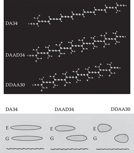
FIGURE 5.13 Schematic wavefunction shapes for DA34, DAAD34, and DDAA30 speculated from the results shown in Figures 5.11 and 5.12.

FIGURE 5.14 Calculated rgn, Δr, and ρβ for DA34, DAAD34, DADA34, and DDAA30. ρβ is β per 1 nm of wire length. From T. Yoshimura, “Enhancing second-order nonlinear optical properties by controlling the wave function in one-dimensional conjugated molecules,” Phys. Rev. B40, 6292–6298 (1989).
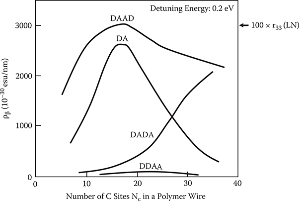
FIGURE 5.15 Calculated ρβ for DA, DAAD, DADA, and DDAA as a function of the number of carbon sites corresponding to the wire length. From T. Yoshimura, “Enhancing second-order nonlinear optical properties by controlling the wave function in one-dimensional conjugated molecules,” Phys. Rev. B40, 6292–6298 (1989).
Thus, it is expected that a large EO effect will be obtained by controlling wave-function dimensionality as well as shapes, which can be realized by adjusting conjugated system lengths and donor–acceptor substitution sites in polymer wires. The maximum optical nonlinearity can be obtained in a dimensionality between zero and one, that is, between a quantum dot condition and a quantum wire condition. For example, in the case of DAAD, maximum optical nonlinearity is obtained in a quantum dot with a length of ~2.2 nm.
5.5.3 RELATIONSHIP BETWEEN WAVEFUNCTIONS AND TRANSITION DIPOLE MOMENTS
To investigate the Nc dependence precisely, the transition dipole moments rgn and Δr are plotted as a function of Nc in Figure 5.16. In DA, rgn increases and Δr decreases with increasing Nc. Consequently, as Figure 5.15 shows, ρβ becomes maximum at an intermediate polymer wire length of Nc = 18. In DAAD, rgn and Δr exhibit Nc dependence similar to DA, with a peak at Nc = 18 in the ρβ versus Nc curve in Figure 5.15. In DADA, Δr and rgn increases with Nc. This is reflected in the increase in ρβ with Nc. In DDAA, rgn is markedly smaller than in the other three types of polymer wires, with ρβ reduced as shown in Figure 5.15.
Because the wavefunction shape affects β via dipole moments, in order to determine the relationship between wavefunctions and β, we must clarify the relationship between the wavefunctions and the dipole moments. As mentioned above, charge separation mainly appears in HOMO and LUMO. Therefore, the G1 -> EN and GM -> E1 composition in Ψn (n = 1) mainly contribute to Δr.
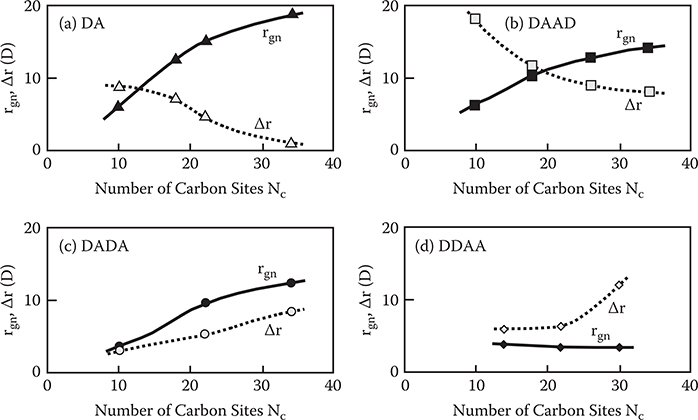
FIGURE 5.16 Dependence of rgn and Δr on the number of carbon sites. From T. Yoshimura, “Enhancing second-order nonlinear optical properties by controlling the wave function in one-dimensional conjugated molecules,” Phys. Rev. B40, 6292–6298 (1989).
In DA, as shown in Figure 5.12(a), the contribution of G1 -> EN and GM -> E1 composition to Ψn is reduced drastically with increasing Nc. This reduces the charge separations, then reduces Δr with increasing Nc. At the same time, the wavefunction overlap between the ground and excited states increases with Nc, enhancing rgn. These results are consistent with Figure 5.16(a). For the DAAD, as Figure 5.12(b) shows, the wavefunction changes similarly to DA with increasing Nc, although not so drastically. This is consistent with Figure 5.16(b). For DA, G1 -> EN and GM -> E1 composition are less than in DAAD, which may account for the fact that in DA, Δr is smaller and rgn is larger than in DAAD (Figures 16(a) and (b)). This is because DA has only one donor and one acceptor, so the electronic pull and push power would be smaller than in DAAD, which has many donors and acceptors.
For DADA, the contribution of the G1 -> EN composition to Ψn remains large when Nc increases from 10 to 34. This enhances Δr (Figure 5.16(c)). For DDAA30, the main composition is the G1 -> EN series and all three orbitals, E1, E2, and E3, exhibit considerable charge separation (Figure 5.11(d)). This increases Δr but reduces rgn because the overlaps of G1/E1, G1/E2, and G1/E3 are small. Thus, rgn in DDAA30 decreases while Δr increases (Figure 5.16(d)).
5.5.4 OPTICAL NONLINEARITY IN CONJUGATED WIRES WITH POLY-AM BACKBONES
So far, enhancement of optical nonlinearities in conjugated wire models with PDA backbones has been described. The same enhancement of optical nonlinearities is found by Matsuura et al. in conjugated wire models with poly-AM backbones [8], which are shown in Figure 5.17 together with calculated βs of the models for 633 nm in wavelength. DDDDAAAA exhibits the largest β, which corresponds to an EO coefficient of 1260 pm/V.
The reason why DDDDAAAA has larger β than AAAADDDD is that N at the edge of the wire has donor-like characteristics. In DDDDAAAA, pull–push strength is increased because the N at the edge and the donor region of DDDD are located on the same side. In AAAADDDD, on the other hand, pull–push strength is suppressed because the N at the edge and the donor region of DDDD are located on the opposite side. Consequently, β in DDDDAAAA becomes larger than β in AAAADDDD.
From of the perspective of polymer wire fabrication by MLD, the poly-AM backbone is useful since MLD of the poly-AM wires has already been demonstrated experimentally as mentioned in Chapters 3 and 4. Possible examples of the MLD process for poly-AM wires with donors and acceptors is shown in Figure 5.18. Five kinds of molecules, molecules A, B, C, D, and E are used. Molecule A is terephthalaldehyde (TPA), and molecule D is p-phenylenediamine (PPDA). Molecule B has two –CHO groups and acceptors. Molecule C has two –CHO groups and donors. Molecule E is for terminating conjugated systems with three single bonds in the molecule. By connecting molecules by MLD in a sequence of molecules A, E, B, D, C, E, …, multiple quantum dot (MQD) structures with donors and acceptors, which is similar to the DDDDAAAA or AAAADDDD structures shown in Figure 5.17, will be constructed.
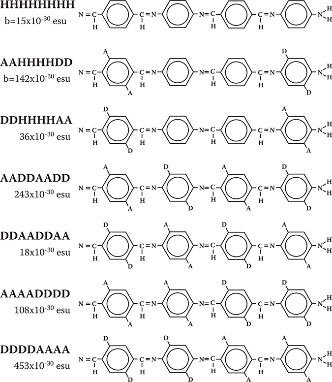
FIGURE 5.17 Models and βs of electro-optic conjugated wires with poly-AM backbones.
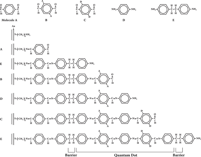
FIGURE 5.18 Possible example of MLD process for poly-AM wires with donors and acceptors.
5.5.5 ENHANCEMENT OF OPTICAL NONLINEARITY BY SHARPENING ABSORPTION BANDS
Figure 5.19 shows the resonant enhancement of ρβ near the first excited state for DAAD18. The absorption band width of polydiacetylene is about 0.1 eV, so a detuning energy of about 0.2 eV is necessary for low-loss operation. In this case, the EO coefficient is about 2 orders of magnitude larger than r33 in LiNbO3. If the band width could be reduced 1 order of magnitude by sharpening the absorption band, the detuning energy required would only be ~0.02 eV, and the EO coefficient would be about 104 times larger than r33 in LiNbO3. This leads us to believe that to improve the nonlinear optical properties in organic materials, sharpening the absorption band [9] is important as well as controlling the wavefunction.
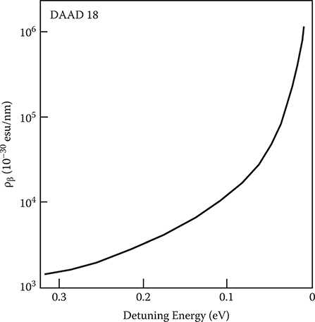
FIGURE 5.19 Photon energy dependence of ρβ in DAAD18. From T. Yoshimura, “Enhancing second-order nonlinear optical properties by controlling the wave function in one-dimensional conjugated molecules,” Phys. Rev. B40, 6292–6298 (1989).
The uniformity of the conjugated length in materials is essential in sharpening. Reducing the exciton–phonon (or electron–phonon) coupling strength is also important. One way to do this might be to use rigid polymer structures. Bound excitons or exciton confinement in quantum dots in one-dimensional conjugated systems may be another way to sharpen absorption bands.
5.6 ENHANCEMENT OF THIRD-ORDER OPTICAL NONLINEARITY BY CONTROLLING WAVEFUNCTIONS
To improve the Kerr effect, which is one of the third-order nonlinear optical effects, the shape of the wavefunction was controlled by constructing quantum dot structures in one-dimensional conjugated systems [3] according to the qualitative guidelines mentioned in Section 5.4. Figures 5.20(a) and (b) give an example of a quantum dot structure and corresponding wavefunctions. Varying the dot length in the conduction band (ML) and that in the valence band (W) adjusts the wavefunction spread difference between the ground and excited states.
D is the dot width. Reducing D changes the system from two-dimensional to one-dimensional. γ per unit length for the light polarization with the well length direction was calculated from Equation (5.33). For simplicity, it was assumed that the ground state wavefunction has even parity, the excited state wavefunction odd parity, and wavefunctions are square waves. The results are shown in Figure 5.20(c). With reduced D, both (r2)e-(r2)g, and rge2 increase, then γ increases rapidly. This clearly indicates that the one-dimensional system is better than a two-dimensional system for inducing large optical nonlinearity, as mentioned in Section 5.2. That is, a wavefunction extending perpendicular to the direction of light polarization contributes little to optical nonlinearity, simply diluting the wavefunction density and reducing optical nonlinearity.
With increasing W, that is, increasing the overlap and decreasing the difference in wavefunction spread between the ground and excited states, rge2 increases and (r2)e-(r2)g decreases, with γ peaking at an intermediate region in W.
Figures 5.21(a) and (b) show a structure and wavefunctions for a double quantum dot (DQD) with subdots at both sides. The wavefunction spread difference is controlled by the difference in dot depth between the conduction band and the valence band. With increasing dot depth, the wavefunction tends to localize on both sides. The calculated values of γ, (r2)e-(r2)g, and rge2 are shown in Figure 5.21(c) as a function of R = C/D. R is a measure of the wavefunction extent in the valence band as defined in Figure 5.21(b). With increasing R, (r2)e-(r2)g increases and rge2 decreases. γ peaks at an intermediate region in R of about 1 when the balance between the wavefunction overlap and the wavefunction spread difference is optimum. In this case, γ is improved about five times over that for a single quantum dot (SQD). It was also found that further confinement of electrons in three or more subdots would make it possible to enhance γ more than ten times.
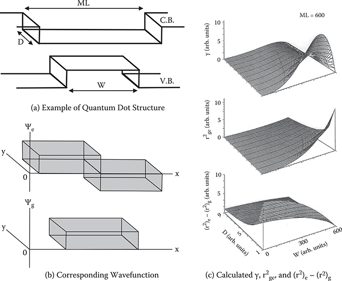
FIGURE 5.20 Enhancement of γ by controlling wavefunction shapes with quantum dot structures.
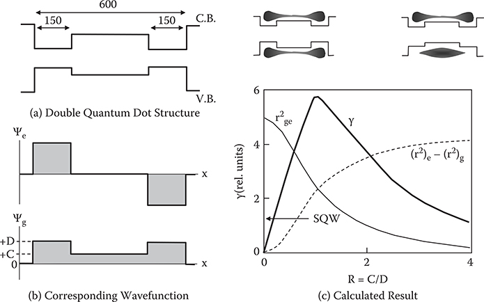
FIGURE 5.21 Enhancement of γ by controlling wavefunction shape in double quantum dot structures.
5.7 Multiple Quantum Dots (MQDS) in Conjugated Polymer Wires
To apply the tailored materials described in Sections 5.5 and 5.6 to practical devices, it is necessary to fabricate the materials in ordered structures. This involves constructing MQD structures in one-dimensional conjugated polymer wires. One way to do this is to insert molecules for cutting the π-conjugation in polymer wires as described in Chapter 4.
The author found another way to form quantum dots [3]. It was simulated by the MO calculation that the energy gap of conjugated polymer wires with PDA backbones is reduced when donors and acceptors are substituted in the DAAD configuration. Figure 5.22 shows one of the examples. The energy gap is decreased from 3.3 eV of the intrinsic PDA wires to 1.6 eV by donor–acceptor substitutions. The phenomena can be used for MQD construction.
The mechanism of the energy gap narrowing in conjugated polymer wires by donor and acceptor substitution is as follows. From the viewpoint of charge distributions, it is found from Figure 5.23 that electrons are localized around donor sites in HOMO while they are localized around acceptor sites in LUMO. The electron distribution in HOMO corresponds to hole distributions in HOMO when the electron is excited. So, with decreasing the distance between donors and acceptors, electron–hole distance becomes short, increasing electric fields in the area, resulting in a large potential energy slope as shown in Figure 5.24. Then, energy gaps become narrow.
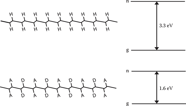
FIGURE 5.22 Energy gap narrowing in conjugated polymer wires by donor and acceptor substitution.
In Figure 5.25, DAAD18 and PDA with an inserted DAAD18 structure are compared. Although wavefunctions slightly penetrate into the barrier regions by tunneling in the conjugated polymer wire with an inserted DAAD18 structure, the molecular orbitals and β are almost the same for both. Therefore, using this effect, it will be possible to insert many DAAD structures into the conjugated polymer wire, constructing a polymer MQD of a polymer superlattice, as shown in Figure 5.26. This structure enables us to align wavefunctions of DAAD structures in the wire direction perfectly, which is favorable to attaining a large Pockels effect.
As mentioned above, using energy gap narrowing, it should be possible to form quantum dots in one-dimensional conjugated wires by modulating the energy gap with selective substitutions of donors and acceptors into the wires. A DQD structure with two 1.4-nm long dots is shown in Figure 5.27 together with an SQD structure. Quantum dots are formed in a PDA wire with 38 carbon sites. Areas with donor and acceptor substitution are quantum dots, and areas with hydrogen substitution are barriers. The energy gap in the quantum dot region is about 1.6 eV, about one half of that in the barrier region. Molecular orbitals show that electrons are spread throughout the conjugated wires in the SQD. In the DQD, electrons tend to be confined to both sides of the wire. Here, note that although electrons are localized on both sides in all E1 , E2, and E3 unoccupied orbitals, they are in the barrier region in the G3 occupied orbital. This suggests that the wavefunction tends to be delocalized throughout the wire more in the valence band than in the conduction band, reproducing the condition in Figure 5.21.
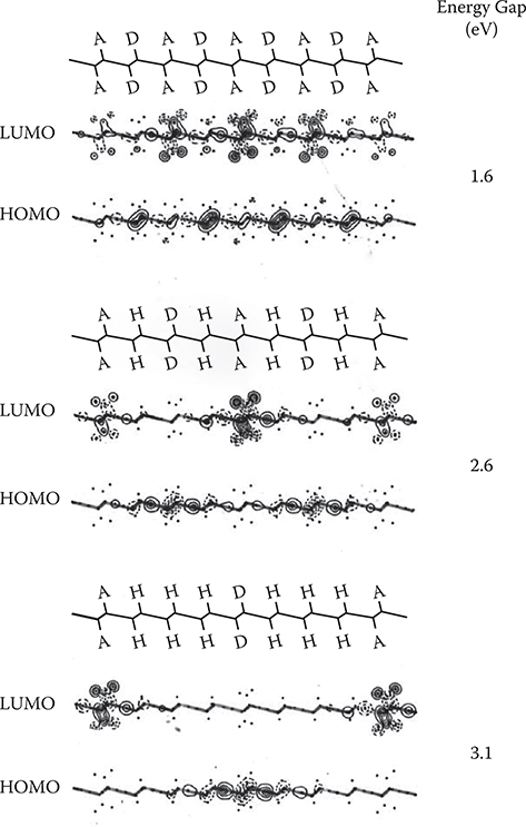
FIGURE 5.23 HOMO and LUMO in conjugated polymer wires with donor and acceptor substitution.
γ of DQD and SQD were calculated by the AM1 MO calculation. As expected, γ in the DQD is more than twice that in the SQD. This confirms that it may be possible to improve third-order optical nonlinearity by adjusting the well structures.
Research on artificial materials, like PDA, poly-AM or other conjugated systems with MQDs, has far-reaching consequences. If a way is developed to connect a molecule on a molecule one by one with direction control, the donor and acceptor substitution locations and the conjugated length could be controlled. MLD is the most promising method for making artificial materials. Figure 5.28 shows possible configurations of EO waveguides consisting of artificial materials fabricated by MLD.
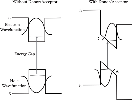
FIGURE 5.24 Mechanism by which the energy gap narrows in conjugated polymer wires by donor and acceptor substitution.
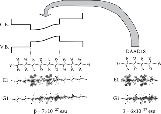
FIGURE 5.25 Insertion of DAAD18 structure into the conjugated polymer wire backbone.
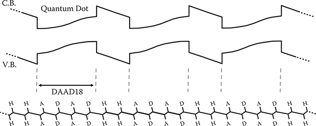
FIGURE 5.26 MQD structure of a polymer superlattice with corresponding electronic potential energy curves.

FIGURE 5.27 SQD and DQD structures and molecular orbitals.

FIGURE 5.28 Possible configurations of EO waveguides consisting of artificial materials fabricated by MLD.
References
1. T. Yoshimura, “Enhancing second-order nonlinear optical properties by controlling the wave function in one-dimensional conjugated molecules,” Phys. Rev. B40, 6292–6298 (1989).
2. T. Yoshimura, “Theoretically predicted influence of donors and acceptors on quadratic hyperpolarizabilities in conjugated long-chain molecules,” Appl. Phys. Lett. 55, 534–536 (1989).
3. T. Yoshimura, “Design of organic nonlinear optical materials for electro-optic and all-optical devices by computer simulation,” FUJITSU Sc. Tech. J. 27, 115–131 (1991).
4. J. Ward, “Calculation of nonlinear optical susceptibilities using diagrammatic perturbation theory,” Rev. Mod. Phys. 37, 1–18 (1965).
5. S. J. Lalama and A. F. Garito, “Origin of the non-linear second-order optical susceptibilities of organic systems,” Phys. Rev. A 20, 1179–1194 (1979).
6. A. F. Garito, C. C. Teng, K. W. Wong, and O. Zammani-Khamiri, “Molecular optics: Nonlinear optical processes in organic and polymer crystals,” Mol. Cryst. Liq. Cryst. 106, 219–258 (1984).
7. J. O. Morley, “Theoretical study of the electronic structure and hyperpolarizabilities of donor-acceptor comulenes and a comparison with the corresponding polyenes and polyynes,” J. Phys. Chem. 99, 10166–10174 (1995).
8. A. Matsuura and T. Hayano, “Theoretical prediction of the donor/acceptor site-dependence on first hyperpolarizabilities in conjugated systems containing azomethine bonds,” Mat. Res. Soc. Symp. Proc. 291, 503–508 (1993).
9. T. Yoshimura, “Estimation of enhancement in third-order nonlinear susceptibility induced by a sharpening absorption band” Opt. Commun. 70, 535–537 (1989).