
Chapter 2. The Technical Context
What I assume you shall assume
—
The discussions in the previous chapter were based on SQL for reasons of familiarity. Unfortunately, however, SQL really isn’t suitable as a basis for the kind of investigation and detailed technical discussion the subject at hand demands. For one thing, the concepts we need to examine often can’t be formulated in SQL at all; for another, even when they can, SQL usually manages to introduce so much irrelevant and unnecessary complexity that it becomes hard to see the forest for the trees, as it were. For such reasons, I intend to use as a foundation for the rest of the book, not SQL as such (though I’ll still have a few things to say about SQL as such from time to time), but rather a hypothetical language called Tutorial D.[13] Now, I believe that language is pretty much self-explanatory; however, a comprehensive description can be found if needed in the book Databases, Types, and the Relational Model: The Third Manifesto, by Hugh Darwen and myself (3rd edition, Addison-Wesley, 2006).[14]
As its title suggests, the book just mentioned—referred to hereinafter as just “the Manifesto book” for short—also introduces and explains The Third Manifesto, a precise though somewhat formal definition of the relational model and a supporting type theory (including, incidentally, a comprehensive model of type inheritance). In that book, we use the name D as a generic name for any language that conforms to the principles laid down by the Manifesto. Any number of distinct languages could qualify as a valid D; sadly, however, SQL isn’t one of them. By contrast, Tutorial D is a valid D, of course; in fact, Tutorial D was explicitly designed to be suitable as a vehicle for illustrating and teaching the ideas of the Manifesto, a state of affairs that makes it equally suitable for the purposes I propose to use it for in this book. Thus, while I’ve said that discussions in this book will be based on Tutorial D, it would really be more accurate to say they’ll be based on the ideas of the Manifesto per se. The remainder of this chapter consists of a survey of those ideas (ignoring, of course, ones that aren’t particularly relevant to our main purpose). In other words, it consists primarily of a summary of material I would really prefer to assume you’re familiar with already. Even if you are, however, it’s probably a good idea at least to give the chapter a “once over lightly” reading anyway, if only to take note of some of the concepts and terminology I’m going to be relying on heavily in subsequent chapters.
Relations and Relvars
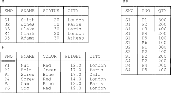
To begin with, then, every relation has a heading and a body, where the heading is a set of attributes and the body is a set of tuples that conform to the heading. For example, referring once again to the suppliers-and-parts database (see Figure 2-1, a repeat of Figure 1-1 from Chapter 1), the heading of the suppliers relation is the set {SNO CHAR, SNAME CHAR, STATUS INTEGER, CITY CHAR}—I’m assuming here for definiteness that attributes SNO, SNAME, STATUS, and CITY are defined to be of types CHAR, CHAR, INTEGER, and CHAR, respectively—and the body of that relation is the set of tuples for suppliers S1, S2, S3, S4, and S5. What’s more, each of those tuples does conform to the pertinent heading, inasmuch as it contains exactly one value, of the applicable type, for each of the attributes SNO, SNAME, STATUS, and CITY (and, of course, nothing else). Note: It would be more precise—and actually more correct—to say that each of those tuples has the pertinent heading, because in fact tuples have headings, just as relations do.
Every relation also has (or is of) a certain type—a certain relation type, to be specific, where the type in question is fully determined by the pertinent heading. Thus, we denote the type of a given relation in Tutorial D by means of the keyword RELATION followed by the applicable heading. For example, here’s the type for the suppliers relation:
RELATION { SNO CHAR , SNAME CHAR , STATUS INTEGER , CITY CHAR }Next, there’s a logical difference between relations as such and relation variables.[15] Take another look at Figure 2-1. That figure shows three relations: namely, the relations that happen to exist in the database at some particular time. But if we were to look at the database at some different time, we would probably see three different relations appearing in their place. In other words, S, P, and SP are really variables—relation variables, to be precise—and like all variables they have different values at different times. And since they’re relation variables specifically, their values at any given time are, of course, relation values. Note, however, that the legal values for a given relation variable must all be of the same relation type—i.e., they must all have the same heading—and the type and heading in question are thereby also considered to be the type and heading of the relation variable as such.
By way of elaboration on the foregoing ideas, suppose the relation variable S currently has the value shown in Figure 2-1, and suppose we delete the tuples for suppliers in London:
DELETE ( S WHERE CITY = 'London' ) FROM S ;
Relation variable S now looks like this:
+-------------------------------+
| SNO | SNAME | STATUS | CITY   |
+-----+-------+--------+--------|
| S2  | Jones |     10 | Paris  |
| S3  | Blake |     30 | Paris  |
| S5  | Adams |     30 | Athens |
+-------------------------------+
Conceptually, what’s happened here is that the old value of S (a relation value, of course) has been replaced in its entirety by a new value (another relation value). Now, the old value (with five tuples) and the new one (with three) are rather similar, in a sense, but they certainly are different values. In fact, the DELETE just shown is logically equivalent to, and is indeed defined to be “shorthand” for,[16] the following relational assignment:
S := S WHERE NOT ( CITY = 'London' ) ;
Or equivalently:
S := S MINUS ( S WHERE CITY = 'London' ) ;
As with all assignments, what happens here is that (a) the source expression on the right side is evaluated and then (b) the value resulting from that evaluation is assigned to the target variable on the left side, with the overall effect already explained.
So DELETE is shorthand for a certain relational assignment—and, of course, an analogous remark applies to INSERT and UPDATE also: They too are basically just shorthand for certain relational assignments. Logically speaking, in fact, relational assignment is the only update operator we really need (a point I’ll elaborate on in the next section).
To sum up: There’s a logical difference between relation values and relation variables. For that reason, I’ll distinguish very carefully between the two from this point forward—I’ll talk in terms of relation values when I mean relation values and relation variables when I mean relation variables. However, I’ll also abbreviate relation value, most of the time, to just relation (exactly as we abbreviate integer value most of the time to just integer). And I’ll abbreviate relation variable most of the time to relvar; for example, I’ll say the suppliers-and-parts database contains three relvars (more specifically, three “real” or base relvars, so called to distinguish them from “virtual” relvars or views).
Base Relvar Definitions
Here for purposes of subsequent reference are Tutorial D definitions for the three base relvars in our running example:
VAR S BASE RELATION
  { SNO CHAR , SNAME CHAR , STATUS INTEGER , CITY CHAR }
    KEY { SNO } ;

VAR P BASE RELATION
  { PNO CHAR , PNAME CHAR , COLOR CHAR , WEIGHT RATIONAL , CITY CHAR }
    KEY { PNO } ;

VAR SP BASE RELATION
  { SNO CHAR , PNO CHAR , QTY INTEGER }
    KEY { SNO , PNO }
    FOREIGN KEY { SNO } REFERENCES S
FOREIGN KEY { PNO } REFERENCES P ;Note: For the purposes of this book, I choose to overlook the fact that Tutorial D as currently defined doesn’t actually include any explicit FOREIGN KEY syntax.
Relational Assignment
The Tutorial D syntax for relational assignment as such—i.e., as opposed to one of the shorthands such as INSERT or DELETE—takes the following generic form:
R:=rx
Here R is a relvar reference (i.e., a relvar name, syntactically speaking), and rx is a relational expression, denoting a relation r, say, of the same type as relvar R. Now, it’s easy to see (thanks to David McGoveran for this observation) that any such assignment is logically equivalent to one of the following form—
R:= (rMINUSd) UNIONi
—where:
r is the “old” value of R
d is a set of tuples to be deleted from R (the “delete set”)
i is a set of tuples to be inserted into R (the “insert set”)[17]
d ⊆ r (i.e., d is a subset of r, meaning we aren’t trying to delete any tuples that don’t exist)
i and r are disjoint (meaning we aren’t trying to insert any tuples that do already exist)
d and i are disjoint a fortiori
d and i are well defined and unique[18]
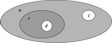
These points can conveniently be illustrated by means of a Venn diagram (see Figure 2-2 overleaf). Explanation: In that diagram, r, d, and i are as above, and u is the universal relation of the pertinent type (in other words, u is the relation whose body consists of all tuples with the same heading as R, including, of course, those tuples that currently appear in R). Note that the difference u – r is the absolute complement of r (in other words, u – r is the relation whose body consists of all tuples with the same heading as R that don’t currently appear in R).
Of course, the delete set d might be empty, in which case the original assignment is effectively a pure INSERT operation. Or the insert set i might be empty, in which case it’s effectively a pure DELETE operation. Or they might both be empty, in which case the assignment overall effectively degenerates to the “no op” R := R.
It follows from all of the above that the original assignment R := rx is in fact logically equivalent to the following multiple assignment (see Multiple Assignment on page 18 for further discussion of this latter construct):[19]
DELETEdFROMR, INSERTiINTOR
As a consequence, although I said earlier that assignment as such is really the only update operator we need, we can always (and for intuitive reasons, at least, it turns out to be convenient to do this) think in terms of DELETE and INSERT operations instead. That is, faced with an arbitrary and possibly multiple assignment to relvar R—including in particular the case where the assignment in question is formulated as an explicit UPDATE on R—I propose that we map that assignment to a DELETE on R and an INSERT on R, where the delete set d and the insert set i are well defined, disjoint, and unique. Note: Because of this state of affairs, in what follows I’ll discuss explicit UPDATE operations only when there’s something interesting to say about them. Also, I’ll ignore for the most part the practical problem of actually computing d and i. My primary concern, in this book as in most of my other writings, is always to get the theory right first before worrying about issues of implementation. Of course, I don’t mean to suggest by these remarks that I think implementation issues are unimportant. Au contraire, in fact—checking feasibility of implementation is crucial to ensuring the correctness of the theory.
A Note on Syntax
To repeat, the assignment R := rx is logically equivalent to the following:
DELETEdFROMR, INSERTiINTOR
Note carefully that it doesn’t matter here whether the DELETE or the INSERT is “done first,” precisely because d and i are disjoint. (I’ll have more to say in a few moments on this question of the order in which the individual operations are done in the context of a multiple assignment.) Thus, we can equally well say that the original assignment is logically equivalent to either of the following:
WITH (R:=RMINUSd) : INSERTiINTORWITH (R:=RUNIONi) : DELETEdFROMR
We could even say it’s logically equivalent to either of the following:
WITH ( DELETEdFROMR) : INSERTiINTORWITH ( INSERTiINTOR) : DELETEdFROMR
Note: If you’re not familiar with WITH specifications as illustrated above, I refer you to SQL and Relational Theory.
In fact we could go further. Tutorial D additionally supports variants on DELETE and INSERT called I_DELETE (“included DELETE”) and D_INSERT (“disjoint INSERT”), respectively. With I_DELETE, it’s an error to attempt to delete a tuple that doesn’t exist (i.e., one that’s not present in the first place); likewise, with D_INSERT, it’s an error to attempt to insert a tuple that does exist (i.e., one that’s already present). Thus, we could actually say the original assignment R := rx is logically equivalent to either of the following:
I_DELETEdFROMR, D_INSERTiINTORD_INSERTiINTOR, I_DELETEdFROMR
For reasons of simplicity and familiarity, however, I’ll stay with the conventional DELETE and INSERT operators throughout the remainder of this book, and I’ll assume throughout the texty—please note carefully!—that an attempt to delete a tuple that doesn’t exist isn’t an error, and nor is an attempt to insert one that does.
Multiple Assignment
The Third Manifesto requires—and as already mentioned,Tutorial D of course supports—a multiple form of assignment, which allows any number of individual assignments to be performed “at the same time.” For example:
DELETE ( S  WHERE SNO = 'S1' ) FROM S ,
DELETE ( SP WHERE SNO = 'S1' ) FROM SP ;
Explanation: First, note the comma separator, which means the two DELETEs are part of the same overall statement. Second, as we know, DELETE is really assignment, and the foregoing “double DELETE” is thus just shorthand for a double assignment of the following general form:
S := ... , SP := ... ;
This latter statement assigns one value to relvar S and another to relvar SP, both as part of the same overall operation. In outline, the semantics of multiple assignment are as follows:
First, the source expressions on the right sides of the individual assignments are evaluated.
Second, those individual assignments are executed.[20]
Observe that, precisely because all of the source expressions are evaluated before any of the individual assignments are executed, none of those individual assignments can depend on the result of any other, and so the sequence in which they’re executed is irrelevant (you can even think of them as being executed in parallel, or “simultaneously,” if you like). Moreover, since multiple assignment is considered to be a semantically atomic operation, no integrity checking is performed “in the middle of” any such assignment (indeed, this state of affairs is the main reason why the Manifesto requires support for the operation in the first place). Note: Integrity constraints are discussed in detail later in this chapter.
Semantics Not Syntax
I’ve said that every relational assignment is equivalent to a DELETE plus an INSERT, where the delete set d and the insert set i are well defined, disjoint, and unique. It’s important to understand, however, that two distinct assignments can use quite different syntax and yet correspond to the same delete set and same insert set, as I’ll now show (thanks to Hugh Darwen for this example).
Consider a relvar R with just two attributes, K and A. Let {K} be the sole key; further, let K and A both be of type INTEGER, and let R contain just two tuples, (1,2) and (3,-2).[21] Now consider the following explicit UPDATE operations:
UPDATE R : { K := K + A } ;

UPDATE R : { A := -A } ;
Note in particular that the first of these is a “key UPDATE” and the second isn’t; thus, if a compensatory action of the form ON UPDATE K … had been defined (which it well might have been, in an SQL context), that action would presumably be invoked in connection with the first UPDATE and not the second. And yet it’s easy to see that, given the specified initial value for R, the two UPDATEs are effectively equivalent—in fact, they’re both equivalent to this explicit assignment:[22]
R := RELATION { TUPLE { K 1 , A -2 } , TUPLE { K 3 , A 2 } } ;In other words, the delete set d is the same for both of the original UPDATEs, and so is the insert set i. (Exercise: What are they, exactly?) Clearly, therefore, what we want is for compensatory actions, if any, to be driven by the applicable delete set and insert set as such, not by the arbitrary choice of syntax in which the pertinent update happens to have been formulated.
Integrity Constraints
Every relvar is subject to a set of integrity constraints, or just constraints for short. First of all, as we know from the section Relations and Relvars, any given relvar is constrained to be of a certain type (more specifically, a certain relation type)—namely, the type specified when the relvar in question is defined. For example, here again is the definition of the suppliers relvar S:[23]
VAR S BASE RELATION
  { SNO CHAR , SNAME CHAR , STATUS INTEGER , CITY CHAR }
    KEY { SNO } ;
As you can see, this definition states explicitly that relvar S is of type RELATION {SNO CHAR, SNAME CHAR, STATUS INTEGER, CITY CHAR}. What’s more, it’s immediate from that specification that attributes SNO, SNAME, STATUS, and CITY are of types CHAR, CHAR, INTEGER, and CHAR, respectively. Note: These latter constraints—the ones on the individual attributes—are examples of what are sometimes called attribute constraints.
To repeat, every relvar (and every attribute, a fortiori) is constrained to be of some type. But relvars in general are also subject to numerous additional constraints, constraints that are typically formulated in Tutorial D by means of explicit CONSTRAINT statements.[24] The following simple examples are, I hope, self-explanatory (further explanation can be found if you need it in SQL and Relational Theory):
CONSTRAINT CX1 IS_EMPTY ( S WHERE STATUS < 1 ) ;

CONSTRAINT CX2 IS_EMPTY ( S WHERE CITY = 'London' AND STATUS ≠ 20 ) ;

CONSTRAINT CX3 IS_EMPTY ( ( S JOIN SP )
                              WHERE STATUS < 20 AND PNO = 'P6' ) ;
Now, The Third Manifesto requires all constraints to be satisfied at statement boundaries (“immediate checking”). In other words, constraints are checked, logically, at the end of any statement that has the potential to violate them.[25] Loosely, we can say they’re checked “at semicolons.” Thus, contrary to the SQL standard and certain SQL products, integrity checking is never deferred to end of transaction or COMMIT time.
Finally, note that it’s sometimes convenient to talk in terms of “the” (total) constraint—sometimes the total relvar constraint, for emphasis—for a given relvar R, meaning the logical AND of all of the individual constraints that mention relvar R. It’s also sometimes convenient to talk in terms of “the” (total) constraint—sometimes the total database constraint, for emphasis—for a given database, meaning the logical AND of all of the constraints that mention any relvar in that database.
Updating Is Set At a Time
The point is well known, but worth stressing nevertheless, that updating in the relational model is always set at a time (better: relation at a time). Loosely speaking, in other words, INSERT inserts a set of tuples into the target relvar; DELETE deletes a set of tuples from the target relvar; UPDATE updates a set of tuples in the target relvar; and, more generally, relational assignment assigns a set of tuples to the target relvar. Of course, it’s true that we often talk in terms of (for example) inserting some individual tuple as such—indeed, I’ll do so myself in this book from time to time—but such a manner of speaking is really sloppy (though convenient). Be that as it may, the significance of the point for present purposes is that no integrity constraint checking must be done until all operations of an updating nature (including compensatory actions, if any) have been completed. In other words, a set level update must not be treated, logically, as a sequence of individual tuple level updates.
Two Important Principles
Now I’m in a position to articulate two important principles that underpin the whole notion of updating in general (including view updating in particular). The first is known as The Golden Rule:
Of course, it’s an immediate consequence of this rule is that no relvar is ever allowed to violate its own total relvar constraint, either. All of which simply amounts to saying, as I’ve already stressed, that constraints must be satisfied at statement boundaries. Note in particular that, to repeat, the rule applies to views just as much as it does to base relvars.
The second principle is called The Assignment Principle:
Definition: The Assignment Principle states that after assignment of value v to variable V, the comparison v = V must evaluate to TRUE.
Now, this principle actually applies to assignments of all kinds—in fact, as I’m sure you realize, it’s more or less the definition of assignment—but for present purposes it’s sufficient to note that it applies to relational assignments in particular. Again note that (of course) the principle applies to views just as much as it does to base relvars.
Relvar Predicates
In Chapter 1, when I introduced the running example (i.e., the suppliers-and-parts database), I said this among other things:
Table S represents suppliers under contract. Each supplier has one supplier number (SNO), unique to that supplier; one name (SNAME), not necessarily unique (though the sample values shown in Figure 1-1 do happen to be unique); one status value (STATUS); and one location (CITY).
Of course, what in that chapter I called “table S” I’d much rather call “relvar S,” but that’s not the point I want to make here. Rather, the point is that, first, the foregoing text represents the meaning of relvar S as understood by the user; second, the term used in logic for such meanings is predicate (or sometimes interpretation or intended interpretation,but I’ll mostly stay with predicate in this book). In other words, we can say of every relvar that it has an associated predicate, called the relvar predicate for the relvar in question, and that relvar predicate is, in essence, how the relvar in question is understood by the user. Here by way of example is the way I would prefer to state the predicate for relvar S:
| S: Supplier SNO is under contract, is named SNAME, has status STATUS, and is located in city CITY. |
And here for the record are the predicates for relvars P and SP:
| P: Part PNO is used in the enterprise, is named PNAME, has color COLOR and weight WEIGHT, and is stored in city CITY. |
| SP: Supplier SNO supplies part PNO in quantity QTY. |
Aside:[26] Perhaps I should say a little more about the way I use the term predicate in this book. First of all, you’re very likely familiar with the term already, since SQL uses it extensively to refer to boolean or truth valued expressions (it talks about comparison predicates, IN predicates, EXISTS predicates, and so on). However, while this usage on SQL’s part isn’t exactly incorrect, it does usurp a very general term—one that’s extremely important in database contexts—and give it a rather specialized meaning, which is why I prefer not to follow that usage myself.
Second, I should explain in the interest of accuracy that a predicate isn’t really a natural language sentence as such, like the ones shown above; rather, it’s the assertion made by such a sentence. For example, the predicate for relvar S is what it is, regardless of whether it’s expressed in English or Spanish or whatever. For simplicity, however, I’ll assume in what follows that a predicate is indeed just a sentence per se, expressed (usually) in some natural language. (Analogous remarks apply to propositions also—see below.)
Finally, I’ve now explained what I mean by the term; however, you should be aware that, the previous paragraph notwithstanding, there seems to be little consensus, even among logicians, as to exactly what a predicate is. In particular, some writers regard a predicate as a purely formal construct that has no meaning in itself, and regard what I’ve referred to above as the intended interpretation as something distinct from the predicate as such. I don’t want to get into arguments about such matters here; for further discussion, I refer you to the article “What’s a Predicate?” in Database Explorations: Essays on The Third Manifesto and Related Topics, by Hugh Darwen and myself (Trafford, 2010). End of aside.
You can think of a predicate as a truth valued function. Like all functions, it has a set of parameters; it returns a result when it’s invoked; and (because it’s truth valued) that result is either TRUE or FALSE. In the case of the predicate for relvar S, for example, the parameters are SNO, SNAME, STATUS, and CITY (corresponding of course to the attributes of the relvar), and they stand for values of the applicable types (CHAR, CHAR, INTEGER, and CHAR, respectively). When we invoke the function—when we instantiate the predicate, as the logicians say—we substitute arguments for the parameters. Suppose we substitute the arguments S1, Smith, 20, and London, respectively. We obtain:
Supplier S1 is under contract, is named Smith, has status 20, and is located in city London.
This latter sentence is in fact a proposition, which in logic is a sentence that has no parameters and evaluates unequivocally to either true or false. (In the case at hand, of course, the proposition is a true one, or so at least we assume for the sake of the example.) Which brings me to another important principle, The Closed World Assumption:
Definition: Let relvar R have predicate P. Then The Closed World Assumption (CWA) says (a) if tuple t appears in R at time T, then the instantiation p of P corresponding to t is assumed to be true at time T; conversely, (b)if tuple t has the same heading as R but doesn’t appear in R at time T, then the instantiation p of P corresponding to t is assumed to be false at time T. In other words, tuple t appears in relvar R at a given time if and only if it satisfies the predicate for R at that time.[27]
For example, with reference to Figure 2-1 once again, it’s currently a “true fact” that supplier S1 supplies part P1 in quantity 300, because the tuple (S1,P1,300) currently appears in relvar SP. But if we were to delete that tuple from that relvar, we would be saying (in effect) that it’s no longer the case that supplier S1 supplies part P1 in quantity 300.
Now, so far I’ve discussed predicates in connection with relvars specifically. In fact, however, all of the foregoing notions extend in a natural way to arbitrary relational expressions. For example, consider the projection of suppliers on all attributes but CITY (note the Tutorial D syntax for projection):[28].
S { SNO , SNAME , STATUS }This expression denotes a relation containing all tuples of the form (s,n,t) such that a tuple of the form (s,n,t,c) currently appears in relvar S for some CITY value c. In other words, the result contains all and only those tuples that correspond to currently true instantiations of the following predicate:
There exists some city CITY such that supplier SNO is under contract, is named SNAME, has status STATUS, and is located in city CITY.
This predicate thus represents the meaning of the expression—the relational expression, that is—S{SNO,SNAME,STATUS}. Observe that it has just three parameters and the corresponding relation has just three attributes; CITY isn’t a parameter to that predicate but what logicians call a “bound variable” instead, owing to the fact that it’s “quantified” by the phrase There exists some city CITY such that. Note: A possibly clearer way of making the same point (i.e., that the predicate has three parameters, not four) is to observe that the predicate in question is effectively equivalent to this one:
Supplier SNO is under contract, is named SNAME, has status STATUS, and is located somewhere [in other words, in some city, but we don’t know which].
Remarks analogous to the foregoing apply to every possible relational expression. To be specific: Every relational expression rx always has an associated meaning, or predicate; moreover, the predicate for rx can always be determined from the predicates for the relvars involved in that expression, in accordance with the semantics of the relational operations involved in that expression.[29]
Aside: To repeat, the projection of suppliers on all attributes but CITY can be expressed in Tutorial D as follows: S {SNO,SNAME,STATUS}. For convenience, however, Tutorial D also allows projections to be expressed in terms of the attributes to be removed instead of the ones to be kept. Thus, for example, the expression S {ALL BUT CITY} is equivalent to the one just shown. An analogous remark applies, where it makes sense, to all of the operators in Tutorial D. End of aside.
Now, relvar predicates as I’ve described them so far are quite informal; in fact, they’re essentially nothing more than a representation in natural language of the fact that the relvar in question has certain attributes (equivalently, is of a certain type). But we could use a somewhat more formal style if we wanted to. For example, given that the suppliers relvar S has attributes SNO, SNAME, STATUS, and CITY, and given also that {SNO} is the sole key for that relvar, we might say the corresponding predicate looks something like this:
is_entity  ( SNO ) AND
has_SNAME  ( SNO , SNAME ) AND
has_STATUS ( SNO , STATUS ) AND
has_CITY   ( SNO , CITY )
Suppose tuple t currently appears in relvar S. Then the foregoing predicate asserts that:
The SNO value in t identifies a certain entity.
That entity has an SNAME property, the value of which is given by the SNAME value in t.
That entity also has a STATUS property, the value of which is given by the STATUS value in t.
That entity also has a CITY property, the value of which is given by the CITY value in t.
Of course, the system still doesn’t know the entity in question (the entity identified by SNO) is in fact a supplier in the real world—a supplier “under contract,” in fact—nor does it know what it means for something to have an SNAME property or a STATUS property or a CITY property.
In a similar manner, we might say the predicate for the projection of suppliers on all attributes but CITY is:
is_entity  ( SNO ) AND
has_SNAME  ( SNO , SNAME ) AND
has_STATUS ( SNO , STATUS ) AND
EXISTS CITY ( has_CITY ( SNO , CITY ) )
Finally, I’d like to close this section by confessing that everything I’ve said so far regarding relvar predicates in general has deliberately been slightly simplified. Of course, I believe the treatment is adequate for present purposes; for further specifics, however—“the true story,” as it were, or at least a slightly truer one—I refer you to Chapter 4 (“The Closed World Assumption”) of my book Logic and Databases: The Roots of Relational Theory (Trafford, 2007).
Matching, not Matching, and Extend
Throughout the bulk of this book, I will of course be discussing the operators of the relational algebra in some detail, and for the most part I’ll take it you’re reasonably familiar already with the operators in question (though definitions can be found if you need them in Appendix B). But there are certain useful operators, supported by Tutorial D in particular, that I do need to appeal to fairly frequently but you might not be familiar with, since they’re not discussed in most of the usual textbooks (probably because they’re not supported by SQL—at least, not directly). The first is MATCHING. Here’s a definition:
Here’s an example (“Get suppliers who currently supply at least one part”):
S MATCHING SP
Given our usual sample values, the result looks like this:
+-------------------------------+
| SNO | SNAME | STATUS | CITY   |
+-----+-------+--------+--------|
| S1  | Smith |     20 | London |
| S2  | Jones |     10 | Paris  |
| S3  | Blake |     30 | Paris  |
| S4  | Clark |     20 | London |
+-------------------------------+
Tutorial D also supports a negated form called NOT MATCHING. Here’s the definition:
Definition: The expression r1 NOT MATCHING r2 returns a relation equal to the relation returned by the expression r1 MINUS (r1 MATCHING r2).[30]
Here’s an example (“Get suppliers who currently supply no parts at all”):
S NOT MATCHING SP
Given our usual sample values, the result looks like this:
+-------------------------------+
| SNO | SNAME | STATUS | CITY   |
+-----+-------+--------+--------|
| S5  | Adams |     30 | Athens |
+-------------------------------+
The other operator I want to describe briefly here is EXTEND. EXTEND comes in two forms. Here’s a definition of the first:
Definition: Let relation r not have an attribute called A. Then the expression EXTEND r : {A := exp} returns a relation with heading the heading of r extended with attribute A and body the set of all tuples t such that t is a tuple of r extended with a value for A that’s computed by evaluating exp on that tuple of r.
By way of example, suppose part weights in relvar P are given in pounds, and we want to see those weights in grams. There are 454 grams to a pound, and so we can write:
EXTEND P : { GMWT := WEIGHT * 454 }
Given our usual sample values, the result looks like this:
+------------------------------------------------+
| PNO | PNAME | COLOR | WEIGHT | CITY   | GMWT   |
+-----+-------+-------+--------+--------+--------|
| P1  | Nut   | Red   |   12.0 | London | 5448.0 |
| P2  | Bolt  | Green |   17.0 | Paris  | 7718.0 |
| P3  | Screw | Blue  |   17.0 | Oslo   | 7718.0 |
| P4  | Screw | Red   |   14.0 | London | 6356.0 |
| P5  | Cam   | Blue  |   12.0 | Paris  | 5448.0 |
| P6  | Cog   | Red   |   19.0 | London | 8626.0 |
+------------------------------------------------+
The second form of EXTEND is aimed primarily at what are sometimes called “what if” queries. In other words, it can be used to explore the effect of making certain changes without actually having to make (and subsequently unmake, possibly) the changes in question. Here’s an example (“What if part weights were given in grams instead of pounds?”):
EXTEND P : { WEIGHT := WEIGHT * 454 }The point here is that the target attribute in the assignment in braces here isn’t a “new” attribute as it was in the previous example; instead, it’s an attribute that already exists in the specified relation (that relation being the current value of relvar P, in the case at hand). The expression overall is defined to be equivalent to the following:
( ( EXTEND P : { GMWT := WEIGHT * 454 } ) { ALL BUT WEIGHT } )
RENAME { GMWT AS WEIGHT }Note: As you can see, this expansion makes use of the Tutorial D RENAME operator. I think that operator is more or less self-explanatory, but you can find a definition if you need it in Appendix B. For further discussion, see SQL and Relational Theory.
For completeness, here’s a definition of this second form of EXTEND:
Definition: Let relation r have an attribute called A. Then the expression EXTEND r : {A := exp} returns a relation with heading the same as that of r and body the set of all tuples t such that t is derived from a tuple of r by replacing the value of A by a value that’s computed by evaluating the expression exp on that tuple of r.
Databases and Dbvars
This is the final section of this chapter. In it, I want to draw your attention to the important fact that just as there’s a logical difference between relation values and relation variables (relvars), so there’s also a logical difference between database values and database variables, or what might be called dbvars. Here’s a quote from the Manifesto book:
The first version of this Manifesto distinguished databases per se (i.e., database values) from database variables … [It also] suggested that the unqualified term database be used to mean a database value specifically, and it introduced the term dbvar as shorthand for “database variable.” While we still believe this distinction to be a valid one, we found it had little direct relevance to other aspects of the Manifesto. We therefore decided, in the interests of familiarity, to revert to more traditional terminology.[31]
It follows that when we “update some relvar” (within some database), what we’re really doing is updating the pertinent dbvar. (For clarity, I’ll adopt the term dbvar for the remainder of this section.) For example, the Tutorial D statement
DELETE ( SP WHERE QTY < 150 ) FROM SP ;
“updates the shipments relvar SP” and thus really updates the entire suppliers-and-parts dbvar—the “new” database value for that dbvar being the same as the “old” one except that certain shipment tuples have been removed. In other words, while we might say a database “contains variables” (namely, the applicable relvars), such a manner of speaking is really only approximate, and is in fact quite informal. A more formal and more accurate way of characterizing the situation is this:
A dbvar is a tuple variable.
The tuple variable in question has one attribute for each relvar in the dbvar (and no other attributes), and each of those attributes is relation valued. In the case of suppliers and parts, for example, we can think of the entire dbvar as a tuple variable (or “tuplevar”) of the following tuple type:
TUPLE { S  RELATION { SNO CHAR , SNAME CHAR ,
                      STATUS INTEGER, CITY CHAR } ,
        P  RELATION { PNO CHAR , PNAME CHAR ,
                      COLOR CHAR , WEIGHT RATIONAL , CITY CHAR } ,
        SP RELATION { SNO CHAR , PNO CHAR , QTY INTEGER } }
Let’s agree, just for the moment, to call the suppliers-and-parts dbvar (or tuplevar, if you prefer) SPDB.[32] Then the DELETE statement shown above can be regarded as shorthand for the following database (and hence tuple) assignment:
SPDB := TUPLE { S  ( S FROM SPDB ) ,
                P  ( P FROM SPDB ) ,
SP ( ( SP FROM SPDB ) WHERE NOT ( QTY < 150 ) ) } ;Explanation: The expression on the right side of this assignment denotes a tuple with three attributes called S, P, and SP, each of which is relation valued.[33] Within that tuple, the value of attribute S is the current value of relvar S; the value of attribute P is the current value of relvar P; and the value of attribute SP is the current value of relvar SP, minus those tuples for which the quantity is less than 150.
By way of another example, here again is the “double delete” I used earlier in this chapter to introduce the concept of multiple assignment:
DELETE ( S  WHERE SNO = 'S1' ) FROM S ,
DELETE ( SP WHERE SNO = 'S1' ) FROM SP ;
Observe now that this relational assignment—which is, of course, a multiple assignment—is logically equivalent to the following single database (and hence tuple) assignment:
SPDB := TUPLE { S  ( ( S FROM SPDB ) WHERE NOT ( SNO = 'S1' ) ,
                P  ( P FROM SPDB ) ,
                SP ( ( SP FROM SPDB ) WHERE NOT ( SNO = 'S1' ) ) } ;
In other words, a multiple assignment in which the target variables are all, specifically, relvars within the same database (or the same dbvar, rather) is merely a syntactic device that allows us to formulate what is logically a database assignment as a collection of separate relational assignments (see further discussion below). And a “single” relational assignment—i.e., a “multiple” relational assignment consisting of just one individual assignment, to one individual database relvar—is nothing but a special case, of course. Fundamentally, in fact, dbvars are the only true variables so far as database updating is concerned; that is, database updates are really always updates to some dbvar as such, and updates via a single database relvar are just a special case.
It follows from the all of the above that even a “single” relational assignment is really a database assignment, if the target relvar is a database relvar (i.e., if that target relvar is a relvar in some database). What’s more, of course, that database assignment, like all assignments, is subject to The Assignment Principle and—because it’s a database assignment in particular—also to The Golden Rule.
The foregoing ideas are so important that it’s worth going over them all again in slightly different words. First of all, then, a dbvar is a tuple variable, and a database (i.e., the value of some given dbvar at some given time) is a tuple in which all of the attributes are relation valued. Second, given a relational assignment of the form
R:=rx
(where R is a relvar reference—i.e., a relvar name, syntactically speaking—that identifies some database relvar and rx is a relational expression, denoting a relation r of the same type as R), that relvar reference R is really a pseudovariable reference (see the remark immediately following this paragraph). In other words, the relational assignment is shorthand for an assignment that “zaps” one component of the corresponding dbvar (which is, to repeat, really a tuple variable). It follows that “relation variables” (at least, relation variables in the database) aren’t really variables as such at all; rather, they’re a convenient fiction that gives the illusion that the database—or dbvar, rather—can be updated piecemeal, individual relvar by individual relvar. And it further follows that, in a sense, “relational assignment” (multiple or otherwise) is also a convenient fiction; to be specific, it’s an operator that lets us pretend that updating a dbvar can be thought of as a collection of updates on individual relvars within that dbvar.[34]
A remark on pseudovariables: Essentially, a pseudovariable reference is a construct—or a symbolic name for such a construct—that looks like an operational expression but, unlike such an expression, doesn’t denote a value; instead, it appears in the target position within some assignment, where it denotes “part of a variable.” For example, let X be a variable of type CHAR, and let the current value of X be ‘antimony’. Then the assignment SUBSTR(X,5,3) := ‘nom’ has the effect of “zapping” the fifth through seventh character positions within X, replacing ‘mon’ by ‘nom’ and thereby replacing the “old” value of X overall (‘antimony’) by a “new” value (‘antinomy’). The construct SUBSTR(X,5,3) on the left side of that assignment is a pseudovariable reference, and the assignment overall is shorthand for X := SUBSTRX(X,1,4) || ‘nom’ || SUBSTR(X,8,1), where the symbol “||” denotes string concatenation. End of remark.
All of that being said, I’ve decided, slightly against my own better judgment, not to use the terminology of database variables and “dbvars” in the remainder of this book—at least, not very much—but rather to stay with the familiar term “database” for both purposes, hoping that my intended meaning will always be clear from the context. Caveat lector.
[13] The language is hypothetical only inasmuch as no commercial implementations exist at the time of writing. But prototype implementations do exist and can be accessed via the website www.thethirdmanifesto.com (see the footnote immediately following).
[14] Tutorial D has been revised and extended somewhat since that book was first published. A description of the revised version (which is close but not identical to the version I’ll be using in this book) can be found in another book by Hugh Darwen and myself, Database Explorations: Essays on The Third Manifesto and Related Topics (Trafford, 2010), as well as on the website www.thethirdmanifesto.com (which, as its name suggests, additionally contains much information concerning the Manifesto as such).
[15] The notion of logical difference, much appealed to by Darwen and myself in technical writings (especially ones to do with The Third Manifesto) derives from a dictum of Wittgenstein’s: All logical differences are big differences.
[16] “Shorthand” in quotation marks because in fact it’s longer than what it’s supposed to be short for. But that’s partly due to the fact that I’m using an unconventional dialect of Tutorial D (the actual Tutorial D syntax for this DELETE would be DELETE S WHERE CITY = ‘London’). The syntax I choose to use for DELETE (and INSERT) in this book is deliberately a trifle verbose, in order that the semantics might be absolutely clear.
[17] Technically, of course, d and i aren’t just “sets of tuples” but in fact relations, of the same type as r.
[18] See Appendix A for a proof of this claim.
[19] The actual Tutorial D syntax for this multiple assignment would be DELETE R d, INSERT R i.
[20] This definition requires some refinement in the case where two or more of the individual assignments specify the same target variable, but that refinement needn’t concern us yet. See Appendix A for further explanation.
[21] Here and elsewhere in this book I adopt this simplified notation for tuples in the interest of readability.
[22] The expression on the right side of this assignment is a relation selector invocation—in fact, a relation literal. Refer to SQL and Relational Theory if you need further explanation of such matters.
[24] The exceptions are constraints formulated by means of KEY and FOREIGN KEY specifications—but even these are essentially just shorthand for constraints that can be expressed, albeit more longwindedly, using explicit CONSTRAINT statements. See SQL and Relational Theory for further discussion of this point.
[25] I’m simplifying slightly here: Constraints to the effect that some relation selector invocation does indeed yield a relation of the required type are checked “even more immediately,” as part of the process of evaluating the relation selector invocation in question. Again, see SQL and Relational Theory for further explanation.
[26] This aside is taken, lightly edited, from Database Design and Relational Theory. Note: I remind you from the preface that throughout this book I use “Database Design and Relational Theory” as an abbreviated form of reference to my book Database Design and Relational Theory: Normal Forms and All That Jazz (O’Reilly, 2012).
[27] I’d like to stress that “if and only if.” It has at least one important corollary. To be specific, let relvars R1 and R2 have predicates P1 and P2, respectively; then if P1 and P2 are both satisfied by the same tuple t, it follows that t must appear in both R1 and R2. (As a rule of thumb, it might be a good idea to ensure that P1 and P2 are specific enough to preclude the foregoing possibility. Note, however, that we’ll see some deliberate violations of this suggested discipline in Chapters Chapter 4 and Chapter 9-11.)
[28] I remark in passing that we find it convenient to give projection the highest precedence of all of the relational operators in Tutorial D
[29] Thus, we can extend The Closed World Assumption as follows: A proposition p is considered to be true at a given time if it corresponds to a tuple t and that tuple t either (a) appears in some database relvar at that time (as already explained) or (b) appears in some relation that can be derived from the relations that are the values of those database relvars at that time. In other words (loosely): Everything stated or implied by the database is true; everything else is false.
[30] I remark in passing that the well known relational difference operator—MINUS in Tutorial D—is a special case of NOT MATCHING. To be specific, r1 NOT MATCHING r2 degenerates to r1 MINUS r2, as you can easily confirm for yourself, if relations r1 and r2 are of the same type. In a sense, therefore, NOT MATCHIG is actually more fundamental than MINUS is.
[31] In other words, we went on to use the term database to mean sometimes a database variable and sometimes a database value, and we didn’t use the terms database variable or dbvar at all. However, it turned out later that, for reasons I don’t want to go into here, this was a very bad decision on our part. (Doing something you know is logically wrong is usually a bad idea.) As for the way I plan to use this terminology in the present book, please see the remainder of this section.
[32] If we’re to be able to write explicit database assignments as in this example, then dbvars will certainly have to have user visible names, which in Tutorial D (at least as currently defined) they don’t.
[33] In fact the expression in question is a tuple selector invocation. Once again, refer to SQL and Relational Theory if you need further explanation of such matters.
[34] It follows from this discussion that multiple relational assignment in particular is extremely important (absent explicit support for database assignment as such); in fact, it’s going to turn out to be absolutely crucial to certain of the view updating rules to be discussed in subsequent chapters. Given this state of affairs, therefore, I have to say that—forgive me for pointing out the obvious here—it’s unfortunate to say the least that SQL doesn’t support that operator.