9	Practical Aspects in Closed-Loop Control

9.1    ROLE, SCHEMATICS

The performance of power converters can be improved with the use of closed-loop control [1,2]. Because the large majority of power converters start from a voltage source, closed-loop current control is very useful (Figure 9.1). Given the operations at high voltages and with high-frequency switching, the implementation of a current control loop faces a series of specific problems. This chapter discusses these problems and attempts to provide solutions.

9.2    CURRENT MEASUREMENT—SYNCHRONIZATION WITH PWM

The most important module in the current closed-loop control relates to current measurement. The main requirements for the sensor and the acquisition system relate to their capability to detect the presence of electrical noise, temperature, and electromagnetic interference (EMI) radiation in the measurement system. A series of dedicated sensors have been developed to overcome these difficulties.

9.2.1    SHUNT RESISTOR

The older solution for current measurement uses a low-value resistor in the current path and measures the voltage drop across it. The shunt resistor’s resistance will likely be in the order of milliohms or microohms, so that only a modest amount of voltage will be dropped at full current. The sensing resistor’s value should be very stable with current level and temperature and should have a small equivalent inductance. For instance, a 1 W, 15 A, 0.005 Ω surface-mount resistor can have as much as 5 nH of package inductance.

The low value of the shunt resistor is comparable to wire-connection resistance, which means voltage is measured across the shunt to avoid detecting the voltage drop across the current-carrying wire connections. Shunts are usually equipped with four connection terminals so that the voltmeter measures only the voltage dropped by the shunt resistance itself, without any stray voltages originating from wire or connection resistance. Such a measurement method, able to avoid errors caused by wire resistance, is called the Kelvin or 4-wire method. The measurement connection wires are insulated from the power wires at the hinge point and are in contact only at the tips where they clasp the wire or terminal of the subject being measured. Thus, current passing through the measurement circuit does not go through the power path and will not create any error-inducing voltage drop along its length. In other words, there is no common path for the measurement and power currents. Shunt resistors with Kelvin contacts have four connections.

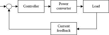
FIGURE 9.1  System diagram for a closed-loop current control.

Shunt resistors are usually made of a low-temperature-coefficient metal foil on an anodized aluminum substrate and can be packaged in either conventional TO-247 or TO-220 packages or SMT packages for lower power level.

Manganin wire (an alloy of copper, manganese, and nickel) has a low temperature coefficient within 15 ppm/°C from 0° to 80°C. Another commonly used low-temperature-coefficient material is nickel–chromium, or nichrome. This has a resistivity of about 110 mV/cm and requires less wire length than manganin’s 44 mV/cm. This helps reduce the inductance for very low-value resistors. Manganin is superior to nichrome in temperature coefficient and long-term stability of resistance value. Another similar alloy is Constantane (Eureka) with a resistivity of 49 mV/cm.

With the advent of Integrated Power Modules during the last decade, several changes occurred with the packaging of lower power level converters as they got more and more on circuit board. This helped integration of thin-film power resistors onto the board layout as individual surface-mount components.

Contemporary designs for low voltage DC/DC converters are using copper traces for building the sensing resistors [3]. The same principles of Kelvin connections are followed and the trace’s length and width are appropriately calculated from knowledge about the material properties. As copper has a high temperature coefficient, additional compensation may be required or operation at elevated temperature may be needed during operation. As we are seeing more and more printed-circuit-board integration of IPM devices, we may see similar designs for the high voltage applications, in the horsepower range. However, accurate designs consider for now dedicated shunt resistors made of low-temperature coefficient materials.

One advantage of the shunt resistor is its practically infinite bandwidth. However, isolation is usually required after the shunt resistor.

The signal from a current-sensing resistor is usually processed with an Operational Amplifier with a high common-mode rejection, as the useful signal is usually floating from ground under a large common-mode voltage. Examples in this class of instrumentation amplifiers include Texas Instrument’s INA148 or INA117 with +200 V common-mode high input, INA146 (100 V cm), INA 149 (275 V cm) or Analog Devices’ AD626. As such devices cannot accommodate a high enough DC common-mode voltage, the sensing resistor should be placed close to ground.

The signal processing usually continues with a low-pass filter implemented around an Operational Amplifier. Among multiple design options, one may consider a second order Bessel-type filter able to allow a constant group delay within the pass-band frequencies, thus providing a lesser waveform distortion [4]. However, the drop of the gain characteristic is less sharp than with Butterworth and Tschebyscheff filter designs. If the switching frequency is rather close to the frequencies of interest, these designs may be more effective. Either way, the actual circuit implementation is recommended to follow the Sallen-Key topology (Figure 9.2).

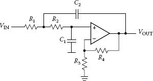
FIGURE 9.2  Sallen-Key topology for low-pass filter on the measurement path.

Another solution for signal processing consists of a high-voltage integrated circuit (IC), such as the IR217x [5]. The IR217x is a monolithic current-sensing high-voltage IC designed for servo-drive applications. It senses the current through an external shunt resistor and modulates a fixed frequency train of pulse with the sensing information. These pulses are transferred to the low side. The output format is a discrete pulse width modulation (PWM) that eliminates the need for an A/D input interface and can be directly connected to a timer circuit within any digital signal processor (DSP) or microcontroller.

Selection and rating of the shunt resistor yield from the trade-off between the desire to have a larger voltage drop for easier signal processing and the allowable power dissipation. A larger voltage drop means a larger resistance that would also produce more power loss across the sensing resistor [6,7].

For a motor drive application, where AC currents are quasi-sinusoidal, it is suggested to select the sensing resistor starting from its power rating (P_max) and the known maximum load (motor) phase current (I_rms). It yields:

•  $R=\frac{P_{\max }}{I_{\text{rms}}^2}$ For a sensing resistor connected directly on the output phase current line:

•  $R=\frac{2\cdot P_{\max }}{I_{\text{rms}}^2}$ For a sensing resistor placed in the emitter of the low-side IGBT:

Similar rating and layout recommendation can be found in [8].

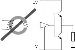
FIGURE 9.3  Open-loop Hall sensor.

9.2.2    HALL EFFECT SENSORS

Shunt resistors are less used today in high-current applications due to the inherent voltage drop. The alternative lies in the use of Hall-effect sensors.

In 1879, Edwin Hall, a graduate student in physics, used a magnetic field to manipulate the charge carriers in a strip of gold foil. He created in the strip a current flowing perpendicular to the field. As the charges that made up the current were moving perpendicular to the field, the magnetic field exerted a force that pushed some of these charges to the top of the strip. Later, scientists discovered the electron and, today, we say that Hall discovered that it was the motion of electrons that caused the current he observed.

An open-loop Hall-effect current sensor is represented in Figure 9.3. It has a block of semiconductor as the sensing element, supplied by a constant current source, and a programmable amplifier to raise the millivolt output to a reasonable value. A current proportional to the measured current is produced in a sensing resistor through the Hall-effect. Older devices used laser-trimmed, thick-film resistors to adjust the programmable amplifier to give a standard output voltage under standard conditions of a magnetic field. Newer devices use a flash memory to hold the amplifier gain setting. A Hall-effect current sensor provides a noise-immune signal and consumes very little power.

Better performance can be achieved with closed-loop current sensors. They represent a different class of Hall-effect current sensors that include an application-specific integrated circuit (ASIC) to provide extremely low offset drift with temperature, resulting in stable, repeatable, accurate measurements.

Hall-effect current sensors are available in hundreds of amperes and provide highly accurate measurement for a large class of power electronic applications. Their bandwidth is usually around 100 kHz, enough for high-power converter applications [9].

9.2.3    CURRENT SENSING TRANSFORMER

For a long time, current-sensing transformers have been considered the best solution for current measurement. The advent of Hall-effect sensing devices, however, reduced the market share of current transformers. They are still used, though, in a limited class of applications, including power converters with high switching frequency. Current-sensing transformers can usually ensure a bandwidth larger than the Hall-effect sensors.

9.2.4    SYNCHRONIZATION WITH PWM

An analog circuit follows the sensor to adapt the range and bandwidth of the signal to the input of the digital circuit. Given the generic inductive type of load, the current will have a quasi-linear variation during each interval characterized by a pulse of voltage.

The current ripple around an average value is determined by the value of inductance, the switching frequency, and the magnitude of the voltage pulse. Sampling the current at any moment during the switching interval introduces a small amount of ripple in the measurement result, leading to aliasing and offset effects (Figure 9.4).

To alleviate these effects, a synchronized PWM is selected to ensure current acquisition during the zero states, when there is no variation in the current and the value already follows the average value of the current. This approach has been recently adopted in the single-phase and three-phase inverter designs, but it is well known from the control of DC/DC converters, such as the phase-shift, full-bridge, zero-voltage switching (ZVS) converter. It has been previously incorporated in a class of Unitrode circuits.

The current sampling synchronized with the PWM signal is used within the Texas Instruments’ family of DSP circuits. This ensures an automatic sampling of the currents or A/D channels at preselected moments when the carrier’s triangular signal changes slopes. In the language of digital circuits, this is equivalent to sampling the analog inputs when the counter reaches the lowest or largest value.

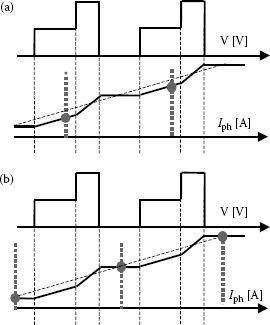
FIGURE 9.4  (a) Current sampling at a random position within the switching interval; (b) synchronized current sampling.

9.3    CURRENT SAMPLING RATE—OVERSAMPLING

As a large majority of modern converters are controlled by digital structures, the conversion of the analog input representing the current into a digital signal should be done at a given sampling rate. The selection of the sampling rate is the result of a compromise among many factors [1,2,10].

First, the power stage switches states at a rate given by the switching frequency. As the goal of the PWM operation is to produce pulses of voltage following a reference signal, sampling current at a rate higher than that of the switching frequency does not have any meaning given the bandwidth limitation at the power stage. Sampling current at the highest frequency possible, that is, the switching frequency of the power stage, may be limited by the real time required to compute the control algorithm.

It is, however, a good practice to sample the current at the highest possible rate even if the control algorithm computes at a lower rate. In this case, we have more samples available than required and this is called oversampling. Oversampling is able to relax the filter requirements in the initial sampling and convert this high rate signal to the desired sample rate using linear digital filters. We basically use the additional samples to filter the final result.

The lowest sampling frequency is determined by the time constants of the electrical circuit or load that influence the performance of the control system. This constraint can also be described as the tracking effectiveness of the control system. The sampling theorem requests sampling at least twice as fast as the highest frequency contained in the signal. If the closed-loop system is required to track a signal with a given bandwidth, the sampling rate should be at least twice the highest frequency in the closed-loop system bandwidth, which can be different from the highest frequency in the plant model. However, defining the lower sampling frequency from the sampling theorem may not satisfy all requirements of the response time of the closed-loop system.

9.4    CURRENT CONTROL IN (a,b,c) COORDINATES

Both motor control and grid applications use the rotating-reference frame to control currents in the so-called d–q system of reference. The current components become quasi-DC and the control is simplified to a low requirement in bandwidth. For a conventional inductive load, the control system reduces to a simple proportional-integral (PI) controller. Variables in the rotating-reference frame must be restored in the stationary three-phase reference frame using inverse transformation.

However, if the system is single-phase or three-phase without an isolated neutral, the control system should be able to track a sinusoidal or harmonic reference. The harmonic reference occurs when the power converter is used within an active filter structure. In either case, the synchronous coordinate transform cannot be applied.

Consider a power converter and load characterized by a plant model G_p(s). The control system is characterized by a transfer function G_C(s). The open-loop transfer function yields:

$G_{OL}(s)=G_c(s)\cdot G_p(s)=\frac{A(s)}{B(s)}$

(9.1)

Considering a sinusoidal reference:

$f(t)=I\cdot \text{ sin ω}t\Rightarrow F(s)=\frac{I\cdot s}{s^2+{\text{ω}}_0^2}$

(9.2)

The error of the feedback signal can be calculated as

$E(s)=\frac{F(s)}{1+G_0(s)}=\frac{B(s)\cdot F(s)}{B(s)+A(s)}=\frac{B(s)}{B(s)+A(s)}\cdot \frac{I\cdot s}{S^2+{\text{ω}}^2}$

(9.3)

Applying the Final Value Theorem defines the constant steady-state value of a time function given its Laplace transform. This uses the partial fraction expansion.

$E(s)=\frac{a_1}{s+{\text{ω}}_1}+\cdots +\frac{a_i}{s+{\text{ω}}_i}+\frac{{\sout{b}}_1}{s-j\cdot {\text{ω}}_0}+\frac{{\sout{b}}_2}{s+j\cdot {\text{ω}}_0}$

(9.4)

If any of the poles ω_i is in the right half of the s-plane, the time-domain signal will increase to an unbounded limit. We will consider these poles with a negative real part. The other pair of imaginary poles derived from the sinusoidal character of the reference would introduce in the time-domain error signal a sinusoidal wave that persists forever and makes impossible the definition of the steady-state error. To avoid this situation, the open-loop transfer function should have the same poles +/− jω₀, so that these poles disappear from the error-transfer function, guaranteeing the reduction of the steady-state error to zero if the signal frequency is well known.

Several solutions are therein possible.

•  Harmonic reference tracking with a P-I-S controller (Figure 9.5) [10]

•  Harmonic reference tracking with a feed-forward controller (Figure 9.6) [11]

Both solutions will be presented in more detail in Chapter 11 for the particular case of AC/DC conversion along with another method based on switching directly the converter states (similar to the hysteretic controller) [12].

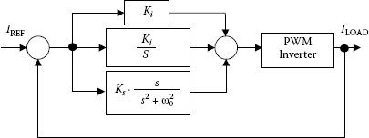
FIGURE 9.5  Current control and harmonic reference tracking with a P-I-S controller.

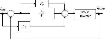
FIGURE 9.6  Current control and harmonic reference tracking with a feed-forward controller.

The stability of the system is, however, dependent on the gain of the s component added to the control system. The transfer function of the open loop exhibits a large phase change around the resonant frequency where the gain is large. The phase margin of the open loop decreases with an increase in the compensation gain. However, a proper selection of the gain can ensure sufficient phase margin.

The problems of tracking a sinusoidal signal can be alleviated with a proper controller, including a term for the effect of the sinusoidal waveform. Despite the success of this solution, current control with reference tracking is more successful in the rotating d–q reference frame. The d and q components are constrained to fix DC values that are easy to control using conventional PI regulators.

Even if the system is either single-phase or three-phase with a connected neutral, the phasor theory can be employed to calculate the d–q components for each phase (independent of the existence of other phases) [13,14].

9.5    CURRENT TRANSFORMS (3->2)—SOFTWARE CALCULATION OF TRANSFORMS

The most common implementation of the current control uses the Park/Clarke set of transforms (Equations 9.5, 9.6, 9.7).

$\left[\begin{array}{c}{I}_{\text{α}}\\ I_{\text{β}}\\ I_0\end{array}\right]=\frac{2}{3}\cdot \left[\begin{array}{ccc}1& -\frac{1}{2}& -\frac{1}{2}\\ 0& \frac{\sqrt{3}}{2}& \frac{\sqrt{3}}{2}\\ \frac{1}{2}& \frac{1}{2}& \frac{1}{2}\end{array}\right]\cdot \left[\begin{array}{c}{i}_X\\ i_Y\\ i_Z\end{array}\right]$

(9.5)

$\left[\begin{array}{c}{I}_d\\ I_q\\ I_0\end{array}\right]=\left[\begin{array}{ccc}\cos \theta & \sin \theta & 0\\ -\sin \theta & \cos \theta & 0\\ 0& 0& 1\end{array}\right]\cdot \left[\begin{array}{c}{I}_{\text{α}}\\ I_{\text{β}}\\ I_0\end{array}\right]$

(9.6)

The same transforms can be grouped within a single form.

$\left[\begin{array}{c}{I}_d\\ I_q\\ I_0\end{array}\right]=\frac{2}{3}\cdot \left[\begin{array}{ccc}\cos \theta & \cos \left[\theta -\frac{2\cdot \text{π}}{3}\right]& \cos \left[\theta -\frac{4\cdot \text{π}}{3}\right]\\ \sin \theta & \sin \left[\theta -\frac{2\cdot \text{π}}{3}\right]& \sin \left[\theta -\frac{4\cdot \text{π}}{3}\right]\\ \frac{1}{2}& \frac{1}{2}& \frac{1}{2}\end{array}\right]\cdot \left[\begin{array}{c}{i}_X\\ i_Y\\ i_Z\end{array}\right]$

(9.7)

These equations are similar to (Equations 5.8, 5.9, 5.10, 5.11) and more details are provided in Chapter 5.

What concerns the software calculation of these transforms (Equations 8.5 through 8.7), dedicated routines are part of any motor control or grid control library. A look-up table of a trigonometric function, optimized for a 90° sector, is used.

Using closed-loop control in (d, q) coordinates often requires a careful look into the load-circuit equations. As the load may include a first-order system (inductance or capacitance), the controlled measure appears under a derivative in the load-circuit equation. The three-phase equations converted in the (d, q) components should take into account the derivative term. This produces a phase shift of 90° changing a real component into an imaginary one or an imaginary one into a real one. These terms should be considered within the control system and they are called cross-coupling terms [12].

9.6    CURRENT CONTROL IN (D, Q)—MODELS—PI CALIBRATION

The generic control system in (d, q) components is shown in Figure 9.7

The PI control system is described mathematically by

$D_c(s)=k_p+\frac{k_p}{T_1\cdot s}$

(9.8)

The time domain equivalent variation results in

$u(t)=k_p\cdot \text{e}(t)+k_I\cdot \underset{0}{\overset{t}{{\displaystyle \int }}}\text{e}(t)\text{d}t$

(9.9)

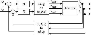
FIGURE 9.7  (d, q) current control of a symmetrical three-phase system.

Considering a linear system, the digital approximation of this equation yields:

$\begin{array}{l}u[k{T}_s+T_s]=k_p\cdot \text{e}[k{T}_s+T_s]+k_I \cdot \underset{0}{\overset{k{T}_s}{{\displaystyle \int }}}\text{e}(t)\text{d}t+k_I\cdot \underset{k{T}_s}{\overset{k{T}_s+T_s}{{\displaystyle \int }}}\text{e}(t)\text{d}t\approx \\ \approx k_p\cdot \text{e}[k{T}_s+T_s]+u_I[k{T}_s]+k_I\cdot \frac{T_s}{2}\cdot \{\text{e}[k{T}_s+T_s]+\text{e}[k{T}_s]\}\end{array}$

(9.10)

There are several ways possible for the approximation of the last integral term. Equation 9.10 is considering an approximation using a trapezoidal form with the base T_s. Furthermore, the calculation of the next action term is usually achieved in one of the following ways:

•  Accumulator method: A large register uI is used as an accumulator for the integral term and the integral component is continuously added to this register. This is the most used method, but its drawback is in the possible windup or overflow of the accumulator.

•  Incremental controller: An incremental controller is used to calculate the change in the action.

$\text{Δ}u=u(k{T}_s+1)-u(k{T}_s)=k_p\cdot (\text{e}[k\cdot T_s+T_s]-\text{e}[k\cdot T_s])+k_I\cdot \text{e}[k\cdot T_s+T_s]$

(9.11)

This implementation is faster and uses a shorter code, but covers the information contained within the accumulator.

In order to design the control system and to define the most appropriate gains for the PI-control system, a model of the load is defined in (d, q) components. Multiple methods are available to develop a controller that will meet given requirements for steady-state and transient response. These methods require a precise dynamic model of the process in the form of equations in motion or a detailed frequency response over a certain range of frequencies. Such methods include:

•  Design with the root locus method

•  Design with the frequency response method

•  Design with the state space method

The design requirements are related to

•  System stability

•  Performance for steady-state operation (steady-state error Err)

•  Performance for dynamic operation (transient time t_p, response time t_r, stabilization time t_s, overshoot M_p) (Figure 9.8)

All of these design methods lead actually to a simplified case for the current control of a mostly inductive load.

In practice, the operator will tune the regulator by trial-and-error. Tuning of the proportional-integral-derivative controllers has been the subject of continuing studies since Callender (1936) [15]. Many of these solutions are based on estimates of the plant model derived from experiment and they can be found in reference textbooks such as [1].

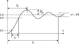
FIGURE 9.8  Parameters of the transient response in time domain.

Ziegler and Nichols provided [16,17] two experimental methods for tuning the PI controller. The first suggests tuning of the control parameters until a decay ratio of 25% is achieved within the step-response transient. This is equivalent to a decay of the transient response to a quarter of its value after one value of oscillation (overshoot). The gains of the PI controller yield k_p = 0.9/RL and TI = L/0.3, where R represents the slope of the step-up response and L represents the lag time at a step change.

Another approach is called the ultimate sensitivity method [1], as it relies on the estimation of the amplitude and frequency of the system oscillations at the limit of stability. The proportional is first increased until the system becomes marginally stable. This can be seen in the existence of continuous oscillations limited by the saturation of the actuator. The gain k and the period T of these oscillations are called the ultimate gain and period. The PI parameters are then calculated as k_p = 0.45k and TI = T/1.2.

9.7    ANTI-WIND-UP PROTECTION—OUTPUT LIMITATION AND RANGE DEFINITION

The real characteristics of the system can cause the actuator to saturate. For instance, a three-phase system has a limited range of the available output voltage, and any requirement from the control system beyond this range would translate in a saturation of the output and loss of controllability. If the error signal continues to be applied to the integrator input under these conditions, the accumulator will grow (wind-up) until the sign of the error changes and the integration turns around. The system behaves as an open-loop system and the accumulator becomes a source of instability in it.

The solution is an integrator antiwind-up circuit, which turns-off the integral action when the actuator saturates. To prevent this, an integrator antiwind-up circuit is used, which turns-off the integral action when the actuator saturates. A simple solution is shown in Figure 9.9.

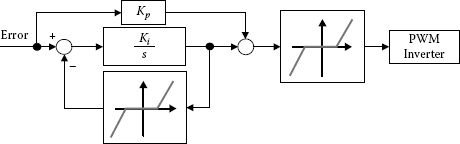
FIGURE 9.9  Anti-windup compensation of a PI controller.

There are many digital control solutions for the implementation of an antiwind-up control system. The system described here shows a linear dependency of the feedback during saturation, which is able to introduce a first-order lag equivalent of an antiwind-up integrator during saturation.

9.8    CONCLUSION

Current control within power converters is subject to noise and distortion. Special precautions need to be taken to filter and measure current in the presence of large ripples. Digital current control is somewhat simple, as a large number of applications use only conventional PI controllers. Several other particular aspects related to implementation are presented in this chapter.

REFERENCES

1.  Franklin, G.F., Powell, J.D., and Emami-Naemi, A. 2002. Feedback Control of Dynamic Systems, Prentice-Hall, Upper Saddle River, NJ.

2.  Ogata, K. 1997. Discrete Time Control Systems. Prentice-Hall, Upper Saddle River, NJ.

3.  Kmetz, J. 1997. Minimum size copper sense resistors. Micrel Application Hint 25.

4.  Mancini, R. 2002. OpAmps for everyone. Application Note SLOD006B, Texas Instruments.

5.  Adams, J. 2003. Using the IR217x linear current sensing ICs. Application Note AN-1052, International Rectifier.

6.  Bille, S.M. 2012. Two or three shunt resistor based current sensing circuit design in 3-phase inverters. ST Microelectronics AN4076. Application Note.

7.  Wood, P., Battello, M., Keskar, N., Guerra, A. 2002. IPM application overview integrated power module for appliance motor drives. Application Note AN-1044.

8.  Anon. 2012. Current sense resistors. Application Note, TT Electronics.

9.  Anon. LEM Sensors. Internet Documentation, www.lemusa.com.

10.  Fukuda, S. and Yoda, T. 2001. A novel current-tracking method for active filters based on a sinusoidal internal model. IEEE Trans. Ind. Appl. 37, 888–894.

11.  Neacsu, D.O. 2010. Analytical investigation of a novel solution to AC waveform tracking control. IEEE International Symposium in Industrial Electronics, Bari, Italy, July 2010, pp. 2684–2689.

12.  Neacsu, D.O. 2004. Current control with fast transient for three-phase AC/DC boost converters. IEEE Trans. Ind. Electron. 51, 1117–1121.

13.  Dong, G. and Ojo, O. 2005. Design issues of natural reference frame current regulators with applications to four-leg converters. IEEE PESC, Recife, Brasil, pp. 1370–1376.

14.  Miranda, U.A., Rolim, L.G.B., and Aredes, M. 2005. A DQ synchronous reference frame current control for single-phase converters. IEEE PESC, Recife, Brasil, pp. 1377–1381.

15.  Callender, A., Hartree, D.R., Porter, A. 1936. Time lag in a control system. Philos. Trans. R. Soc. London A, 235, 415–444.

16.  Ziegler, J.G. and Nichols, N.B. 1942. Optimum settings for automatic controllers. Trans. ASME 64, 759–768.

17.  Ziegler, J.G. and Nichols, N.B. 1943. Process lags in automatic control circuits. Trans. ASME 65(5), 433–444.