
Chapter 6
Transformation Matrices
The machinery of linear algebra can be used to express many of the operations required to arrange objects in a 3D scene, view them with cameras, and get them onto the screen. Geometric transformations like rotation, translation, scaling, and projection can be accomplished with matrix multiplication, and the transformation matrices used to do this are the subject of this chapter.
We will show how a set of points transforms if the points are represented as offset vectors from the origin, and we will use the clock shown in Figure 6.1 as an example of a point set. So think of the clock as a bunch of points that are the ends of vectors whose tails are at the origin. We also discuss how these transforms operate differently on locations (points), displacement vectors, and surface normal vectors.

Scaling uniformly by half for each axis: The axis-aligned scale matrix has the proportion of change in each of the diagonal elements and zeroes in the off-diagonal elements.
6.1 2D Linear Transformations
We can use a 2 × 2 matrix to change, or transform, a 2D vector:
This kind of operation, which takes in a 2-vector and produces another 2-vector by a simple matrix multiplication, is a linear transformation.
By this simple formula we can achieve a variety of useful transformations, depending on what we put in the entries of the matrix, as will be discussed in the following sections. For our purposes, consider moving along the x-axis a horizontal move and along the y-axis, a vertical move.
6.1.1 Scaling
The most basic transform is a scale along the coordinate axes. This transform can change length and possibly direction:
Note what this matrix does to a vector with Cartesian components (x, y):
So, just by looking at the matrix of an axis-aligned scale, we can read off the two scale factors.
Example.
The matrix that shrinks x and y uniformly by a factor of two is (Figure 6.1)
A matrix which halves in the horizontal and increases by three-halves in the vertical is (see Figure 6.2)

Scaling nonuniformly in x and y: The scaling matrix is diagonal with non-equal elements. Note that the square outline of the clock becomes a rectangle and the circular face becomes an ellipse.
6.1.2 Shearing
A shear is something that pushes things sideways, producing something like a deck of cards across which you push your hand; the bottom card stays put and cards move more the closer they are to the top of the deck. The horizontal and vertical shear matrices are
Example.
The transform that shears horizontally so that vertical lines become 45° lines leaning toward the right is (see Figure 6.3)

An x-shear matrix moves points to the right in proportion to their y-coordinate. Now the square outline of the clock becomes a parallelogram and, as with scaling, the circular face of the clock becomes an ellipse.
An analogous transform vertically is (see Figure 6.4)

In both cases, the square outline of the sheared clock becomes a parallelogram, and the circular face of the sheared clock becomes an ellipse.
Another way to think of a shear is in terms of rotation of only the vertical (or horizontal) axis. The shear transform that takes a vertical axis and tilts it clockwise by an angle ϕ is
Similarly, the shear matrix which rotates the horizontal axis counterclockwise by angle ϕ is
6.1.3 Rotation
Suppose we want to rotate a vector a by an angle ϕ counterclockwise to get vector b (Figure 6.5). If a makes an angle α with the x-axis, and its length is , then we know that

Because b is a rotation of a, it also has length r. Because it is rotated an angle ϕ from a, b makes an angle (α + ϕ) with the x-axis. Using the trigonometric addition identities (Section 2.3.3):
Substituting xa = r cos α and ya = r sin α gives
In matrix form, the transformation that takes a to b is then
Example
A matrix that rotates vectors by π/4 radians (45 degrees) is (see Figure 6.6)

A rotation by 45°. Note that the rotation is counterclockwise and that cos(45°) = sin(45°) ≈ .707.
A matrix that rotates by π/6 radians (30 degrees) in the clockwise direction is a rotation by −π/6 radians in our framework (see Figure 6.7):

A rotation by −30 degrees. Note that the rotation is clockwise and that cos(−30°) ≈ .866 and sin(−30°) = −.5.
Because the norm of each row of a rotation matrix is one (sin2ϕ+cos2ϕ = 1), and the rows are orthogonal (cos ϕ(−sin ϕ) + sin ϕ cos ϕ = 0), we see that rotation matrices are orthogonal matrices (Section 5.2.4). By looking at the matrix we can read off two pairs of orthonormal vectors: the two columns, which are the vectors to which the transformation sends the canonical basis vectors (1, 0) and (0, 1); and the rows, which are the vectors that the transformations sends to the canonical basis vectors.
6.1.4 Reflection
We can reflect a vector across either of the coordinate axes by using a scale with one negative scale factor (see Figures 6.8 and 6.9):


While one might expect that the matrix with −1 in both elements of the diagonal is also a reflection, in fact it is just a rotation by π radians.
6.1.5 Composition and Decomposition of Transformations
It is common for graphics programs to apply more than one transformation to an object. For example, we might want to first apply a scale S, and then a rotation R. This would be done in two steps on a 2D vector v1:
Another way to write this is
Because matrix multiplication is associative, we can also write
In other words, we can represent the effects of transforming a vector by two matrices in sequence using a single matrix of the same size, which we can compute by multiplying the two matrices: M = RS (Figure 6.10).

Applying the two transform matrices in sequence is the same as applying the product of those matrices once. This is a key concept that underlies most graphics hardware and software.
It is very important to remember that these transforms are applied from the right side first. So the matrix M = RS first applies S and then R.
Suppose we want to scale by one-half in the vertical direction and then rotate by π/4 radians (45 degrees). The resulting matrix is
It is important to always remember that matrix multiplication is not commutative. So the order of transforms does matter. In this example, rotating first, and then scaling, results in a different matrix (see Figure 6.11):
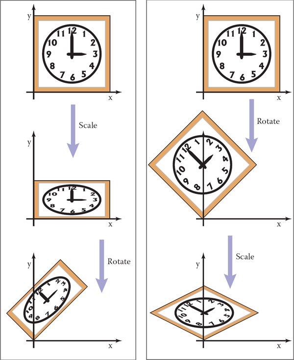
The order in which two transforms are applied is usually important. In this example, we do a scale by one-half in y and then rotate by 45°. Reversing the order in which these two transforms are applied yields a different result.
Example.
Using the scale matrices we have presented, nonuniform scaling can only be done along the coordinate axes. If we wanted to stretch our clock by 50% along one of its diagonals, so that 8:00 through 1:00 move to the northwest and 2:00 through 7:00 move to the southeast, we can use rotation matrices in combination with an axis-aligned scaling matrix to get the result we want. The idea is to use a rotation to align the scaling axis with a coordinate axis, then scale along that axis, then rotate back. In our example, the scaling axis is the “backslash” diagonal of the square, and we can make it parallel to the x-axis with a rotation by +45°. Putting these operations together, the full transformation is
In mathematical notation, this can be written RSRT. The result of multiplying the three matrices together is
Building up a transformation from rotation and scaling transformations actually works for any linear transformation, and this fact leads to a powerful way of thinking about these transformations, as explored in the next section.
6.1.6 Decomposition of Transformations
Sometimes it’s necessary to “undo” a composition of transformations, taking a transformation apart into simpler pieces. For instance, it’s often useful to present a transformation to the user for manipulation in terms of separate rotations and scale factors, but a transformation might be represented internally simply as a matrix, with the rotations and scales already mixed together. This kind of manipulation can be achieved if the matrix can be computationally disassembled into the desired pieces, the pieces adjusted, and the matrix reassembled by multiplying the pieces together again.
It turns out that this decomposition, or factorization, is possible, regardless of the entries in the matrix—and this fact provides a fruitful way of thinking about transformations and what they do to geometry that is transformed by them.
Symmetric Eigenvalue Decomposition
Let’s start with symmetric matrices. Recall from Section 5.4 that a symmetric matrix can always be taken apart using the eigenvalue decomposition into a product of the form
where R is an orthogonal matrix and S is a diagonal matrix; we will call the columns of R (the eigenvectors) by the names v1 and v2, and we’ll call the diagonal entries of S (the eigenvalues) by the names λ1 and λ2.
In geometric terms we can now recognize R as a rotation and S as a scale, so this is just a multi-step geometric transformation (Figure 6.13):

What happens when the unit circle is transformed by an arbitrary symmetric matrix A, also known as a non–axis-aligned, nonuniform scale. The two perpendicular vectors v1 and v2, which are the eigenvectors of A, remain fixed in direction but get scaled. In terms of elementary transformations, this can be seen as first rotating the eigenvectors to the canonical basis, doing an axis-aligned scale, and then rotating the canonical basis back to the eigenvectors.
- Rotate v1 and v2 to the x- and y-axes (the transform by RT).
- Scale in x and y by (λ1, λ2) (the transform by S).
- Rotate the x- and y-axes back to v1 and v2 (the transform by R).
Looking at the effect of these three transforms together, we can see that they have the effect of a nonuniform scale along a pair of axes. As with an axis-aligned scale, the axes are perpendicular, but they aren’t the coordinate axes; instead they are the eigenvectors of A. This tells us something about what it means to be a symmetric matrix: symmetric matrices are just scaling operations—albeit potentially nonuniform and non-axis-aligned ones.
Example.
Recall the example from Section 5.4:
The matrix above, then, according to its eigenvalue decomposition, scales in a direction 31.7° counterclockwise from three o’clock (the x-axis). This is a touch before 2 p.m. on the clockface as is confirmed by Figure 6.14.

A symmetric matrix is always a scale along some axis. In this case it is along the ϕ = 31.7° direction which means the real eigenvector for this matrix is in that direction.
We can also reverse the diagonalization process; to scale by (λ1, λ2) with the first scaling direction an angle ϕ clockwise from the x-axis, we have
We should take heart that this is a symmetric matrix as we know must be true since we constructed it from a symmetric eigenvalue decomposition.
Singular Value Decomposition
A very similar kind of decomposition can be done with nonsymmetric matrices as well: it’s the Singular Value Decomposition (SVD), also discussed in Section 5.4.1. The difference is that the matrices on either side of the diagonal matrix are no longer the same:
The two orthogonal matrices that replace the single rotation R are called U and V, and their columns are called ui (the left singular vectors) and vi (the right singular vectors), respectively. In this context, the diagonal entries of S are called singular values rather than eigenvalues. The geometric interpretation is very similar to that of the symmetric eigenvalue decomposition (Figure 6.15):
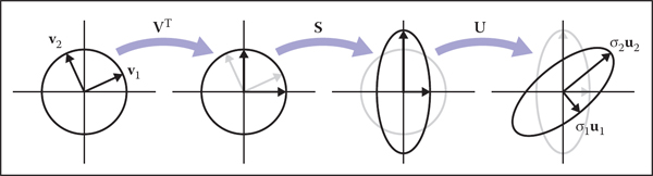
What happens when the unit circle is transformed by an arbitrary matrix A. The two perpendicular vectors v1 and v2, which are the right singular vectors of A, get scaled and changed in direction to match the left singular vectors, u1 and u2. In terms of elementary transformations, this can be seen as first rotating the right singular vectors to the canonical basis, doing an axis-aligned scale, and then rotating the canonical basis to the left singular vectors.
- Rotate v1 and v2 to the x- and y-axes (the transform by VT).
- Scale in x and y by (σ1, σ2) (the transform by S).
- Rotate the x- and y-axes to u1 and u2 (the transform by U).
The principal difference is between a single rotation and two different orthogonal matrices. This difference causes another, less important, difference. Because the SVD has different singular vectors on the two sides, there is no need for negative singular values: we can always flip the sign of a singular value, reverse the direction of one of the associated singular vectors, and end up with the same transformation again. For this reason, the SVD always produces a diagonal matrix with all positive entries, but the matrices U and V are not guaranteed to be rotations—they could include reflection as well. In geometric applications like graphics this is an inconvenience, but a minor one: it is easy to differentiate rotations from reflections by checking the determinant, which is +1 for rotations and −1 for reflections, and if rotations are desired, one of the singular values can be negated, resulting in a rotation-scale-rotation sequence where the reflection is rolled in with the scale, rather than with one of the rotations.
Example.
The example used in Section 5.4.1 is in fact a shear matrix (Figure 6.12):

Singular Value Decomposition (SVD) for a shear matrix. Any 2D matrix can be decomposed into a product of rotation, scale, rotation. Note that the circular face of the clock must become an ellipse because it is just a rotated and scaled circle.
An immediate consequence of the existence of SVD is that all the 2D transformation matrices we have seen can be made from rotation matrices and scale matrices. Shear matrices are a convenience, but they are not required for expressing transformations.
In summary, every matrix can be decomposed via SVD into a rotation times a scale times another rotation. Only symmetric matrices can be decomposed via eigenvalue diagonalization into a rotation times a scale times the inverse-rotation, and such matrices are a simple scale in an arbitrary direction. The SVD of a symmetric matrix will yield the same triple product as eigenvalue decomposition via a slightly more complex algebraic manipulation.
Paeth Decomposition of Rotations
Another decomposition uses shears to represent nonzero rotations (Paeth, 1990). The following identity allows this:
For example, a rotation by π/4 (45 degrees) is (see Figure 6.16)

Any 2D rotation can be accomplished by three shears in sequence. In this case a rotation by 45° is decomposed as shown in Equation 6.2.
This particular transform is useful for raster rotation because shearing is a very efficient raster operation for images; it introduces some jagginess, but will leave no holes. The key observation is that if we take a raster position (i, j) and apply a horizontal shear to it, we get
If we round sj to the nearest integer, this amounts to taking each row in the image and moving it sideways by some amount—a different amount for each row. Because it is the same displacement within a row, this allows us to rotate with no gaps in the resulting image. A similar action works for a vertical shear. Thus, we can implement a simple raster rotation easily.
6.2 3D Linear Transformations
The linear 3D transforms are an extension of the 2D transforms. For example, a scale along Cartesian axes is
Rotation is considerably more complicated in 3D than in 2D, because there are more possible axes of rotation. However, if we simply want to rotate about the z-axis, which will only change x- and y-coordinates, we can use the 2D rotation matrix with no operation on z:
Similarly we can construct matrices to rotate about the x-axis and the y-axis:
We will discuss rotations about arbitrary axes in the next section.
As in two dimensions, we can shear along a particular axis, for example,
As with 2D transforms, any 3D transformation matrix can be decomposed using SVD into a rotation, scale, and another rotation. Any symmetric 3D matrix has an eigenvalue decomposition into rotation, scale, and inverse-rotation. Finally, a 3D rotation can be decomposed into a product of 3D shear matrices.
6.2.1 Arbitrary 3D Rotations
As in 2D, 3D rotations are orthogonal matrices. Geometrically, this means that the three rows of the matrix are the Cartesian coordinates of three mutually orthogonal unit vectors as discussed in Section 2.4.5. The columns are three, potentially different, mutually orthogonal unit vectors. There are an infinite number of such rotation matrices. Let’s write down such a matrix:
Here, u = xux + yuy + zuz and so on for v and w. Since the three vectors are orthonormal we know that
We can infer some of the behavior of the rotation matrix by applying it to the vectors u, v and w. For example,
Note that those three rows of Ruvwu are all dot products:
Similarly, Ruvwv = y, and Ruvww = z. So Ruvw takes the basis uvw to the corresponding Cartesian axes via rotation.
If Ruvw is a rotation matrix with orthonormal rows, then is also a rotation matrix with orthonormal columns, and in fact is the inverse of Ruvw (the inverse of an orthogonal matrix is always its transpose). An important point is that for transformation matrices, the algebraic inverse is also the geometric inverse. So if Ruvw takes u to x, then takes x to u. The same should be true of v and y as we can confirm:
So we can always create rotation matrices from orthonormal bases.
If we wish to rotate about an arbitrary vector a, we can form an orthonormal basis with w = a, rotate that basis to the canonical basis xyz, rotate about the z-axis, and then rotate the canonical basis back to the uvw basis. In matrix form, to rotate about the w-axis by an angle ϕ:
Here we have w a unit vector in the direction of a (i.e., a divided by its own length). But what are u and v? A method to find reasonable u and v is given in Section 2.4.6.
If we have a rotation matrix and we wish to have the rotation in axis-angle form, we can compute the one real eigenvalue (which will be λ = 1), and the corresponding eigenvector is the axis of rotation. This is the one axis that is not changed by the rotation.
See Chapter 16 for a comparison of the few most-used ways to represent rotations, besides rotation matrices.
6.2.2 Transforming Normal Vectors
While most 3D vectors we use represent positions (offset vectors from the origin) or directions, such as where light comes from, some vectors represent surface normals. Surface normal vectors are perpendicular to the tangent plane of a surface. These normals do not transform the way we would like when the underlying surface is transformed. For example, if the points of a surface are transformed by a matrix M, a vector t that is tangent to the surface and is multiplied by M will be tangent to the transformed surface. However, a surface normal vector n that is transformed by M may not be normal to the transformed surface (Figure 6.17).

When a normal vector is transformed using the same matrix that transforms the points on an object, the resulting vector may not be perpendicular to the surface as is shown here for the sheared rectangle. The tangent vector, however, does transform to a vector tangent to the transformed surface.
We can derive a transform matrix N which does take n to a vector perpendicular to the transformed surface. One way to attack this issue is to note that a surface normal vector and a tangent vector are perpendicular, so their dot product is zero, which is expressed in matrix form as
If we denote the desired transformed vectors as tM = Mt and nN = Nn, our goal is to find N such that . We can find N by some algebraic tricks. First, we can sneak an identity matrix into the dot product, and then take advantage of M−1M = I:
Although the manipulations above don’t obviously get us anywhere, note that we can add parentheses that make the above expression more obviously a dot product:
This means that the row vector that is perpendicular to tM is the left part of the expression above. This expression holds for any of the tangent vectors in the tangent plane. Since there is only one direction in 3D (and its opposite) that is perpendicular to all such tangent vectors, we know that the left part of the expression above must be the row vector expression for nN, i.e., it is , so this allows us to infer N:
so we can take the transpose of that to get
Therefore, we can see that the matrix which correctly transforms normal vectors so they remain normal is N = (M−1)T, i.e., the transpose of the inverse matrix. Since this matrix may change the length of n, we can multiply it by an arbitrary scalar and it will still produce nN with the right direction. Recall from Section 5.3 that the inverse of a matrix is the transpose of the cofactor matrix divided by the determinant. Because we don’t care about the length of a normal vector, we can skip the division and find that for a 3 × 3 matrix,
This assumes the element of M in row i and column j is mij. So the full expression for N is
6.3 Translation and Affine Transformations
We have been looking at methods to change vectors using a matrix M. In two dimensions, these transforms have the form,
We cannot use such transforms to move objects, only to scale and rotate them. In particular, the origin (0, 0) always remains fixed under a linear transformation. To move, or translate, an object by shifting all its points the same amount, we need a transform of the form,
There is just no way to do that by multiplying (x, y) by a 2 × 2 matrix. One possibility for adding translation to our system of linear transformations is to simply associate a separate translation vector with each transformation matrix, letting the matrix take care of scaling and rotation and the vector take care of translation. This is perfectly feasible, but the bookkeeping is awkward and the rule for composing two transformations is not as simple and clean as with linear transformations.
Instead, we can use a clever trick to get a single matrix multiplication to do both operations together. The idea is simple: represent the point (x, y) by a 3D vector [x y 1]T, and use 3 × 3 matrices of the form
The fixed third row serves to copy the 1 into the transformed vector, so that all vectors have a 1 in the last place, and the first two rows compute x' and y' as linear combinations of x, y, and 1:
The single matrix implements a linear transformation followed by a translation! This kind of transformation is called an affine transformation, and this way of implementing affine transformations by adding an extra dimension is called homogeneous coordinates (Roberts, 1965; Riesenfeld, 1981; Penna & Patterson, 1986). Homogeneous coordinates not only clean up the code for transformations, but this scheme also makes it obvious how to compose two affine transformations: simply multiply the matrices.
A problem with this new formalism arises when we need to transform vectors that are not supposed to be positions—they represent directions, or offsets between positions. Vectors that represent directions or offsets should not change when we translate an object. Fortunately, we can arrange for this by setting the third coordinate to zero:
If there is a scaling/rotation transformation in the upper-left 2 × 2 entries of the matrix, it will apply to the vector, but the translation still multiplies with the zero and is ignored. Furthermore, the zero is copied into the transformed vector, so direction vectors remain direction vectors after they are transformed.
This is exactly the behavior we want for vectors, so they fit smoothly into the system: the extra (third) coordinate will be either 1 or 0 depending on whether we are encoding a position or a direction. We actually do need to store the homogeneous coordinate so we can distinguish between locations and other vectors. For example,
Later, when we do perspective viewing, we will see that it is useful to allow the homogeneous coordinate to take on values other than one or zero.
Homogeneous coordinates are used nearly universally to represent transformations in graphics systems. In particular, homogeneous coordinates underlie the design and operation of renderers implemented in graphics hardware. We will see in Chapter 7 that homogeneous coordinates also make it easy to draw scenes in perspective, another reason for their popularity.
Homogeneous coordinates can be considered just a clever way to handle the bookkeeping for translation, but there is also a different, geometric interpretation. The key observation is that when we do a 3D shear based on the z-coordinate we get this transform:
Note that this almost has the form we want in x and y for a 2D translation, but has a z hanging around that doesn’t have a meaning in 2D. Now comes the key decision: we will add a coordinate z = 1 to all 2D locations. This gives us
By associating a (z = 1)-coordinate with all 2D points, we now can encode translations into matrix form. For example, to first translate in 2D by (xt, yt) and then rotate by angle ϕ we would use the matrix
Note that the 2D rotation matrix is now 3 × 3 with zeros in the “translation slots.” With this type of formalism, which uses shears along z = 1 to encode translations, we can represent any number of 2D shears, 2D rotations, and 2D translations as one composite 3D matrix. The bottom row of that matrix will always be (0, 0, 1), so we don’t really have to store it. We just need to remember it is there when we multiply two matrices together.
In 3D, the same technique works: we can add a fourth coordinate, a homogeneous coordinate, and then we have translations:
Again, for a direction vector, the fourth coordinate is zero and the vector is thus unaffected by translations.
Example (Windowing transformations).
Often in graphics we need to create a transform matrix that takes points in the rectangle [xl, xh] × [yl, yh] to the rectangle . This can be accomplished with a single scale and translate in sequence. However, it is more intuitive to create the transform from a sequence of three operations (Figure 6.18):

To take one rectangle (window) to the other, we first shift the lower-left corner to the origin, then scale it to the new size, and then move the origin to the lower-left corner of the target rectangle.
- Move the point (xl, yl) to the origin.
- Scale the rectangle to be the same size as the target rectangle.
- Move the origin to point .
Remembering that the right-hand matrix is applied first, we can write
It is perhaps not surprising to some readers that the resulting matrix has the form it does, but the constructive process with the three matrices leaves no doubt as to the correctness of the result.
An exactly analogous construction can be used to define a 3D windowing transformation, which maps the box [xl, xh] × [yl, yh] × [zl, zh] to the box :
It is interesting to note that if we multiply an arbitrary matrix composed of scales, shears, and rotations with a simple translation (translation comes second), we get
Thus, we can look at any matrix and think of it as a scaling/rotation part and a translation part because the components are nicely separated from each other.
An important class of transforms are rigid-body transforms. These are composed only of translations and rotations, so they have no stretching or shrinking of the objects. Such transforms will have a pure rotation for the aij above.
6.4 Inverses of Transformation Matrices
While we can always invert a matrix algebraically, we can use geometry if we know what the transform does. For example, the inverse of scale(sx, sy, sz) is scale(1/sx, 1/sy, 1/sz). The inverse of a rotation is the same rotation with the opposite sign on the angle. The inverse of a translation is a translation in the opposite direction. If we have a series of matrices M = M1M2 ... Mn then
Also, certain types of transformation matrices are easy to invert. We’ve already mentioned scales, which are diagonal matrices; the second important example is rotations, which are orthogonal matrices. Recall (Section 5.2.4) that the inverse of an orthogonal matrix is its transpose. This makes it easy to invert rotations and rigid body transformations (see Exercise 6). Also, it’s useful to know that a matrix with [0 0 0 1] in the bottom row has an inverse that also has [0 0 0 1] in the bottom row (see Exercise 7).
Interestingly, we can use SVD to invert a matrix as well. Since we know that any matrix can be decomposed into a rotation times a scale times a rotation, inversion is straightforward. For example, in 3D we have
and from the rules above it follows easily that
6.5 Coordinate Transformations
All of the previous discussion has been in terms of using transformation matrices to move points around. We can also think of them as simply changing the coordinate system in which the point is represented. For example, in Figure 6.19, we see two ways to visualize a movement. In different contexts, either interpretation may be more suitable.

The point (2,1) has a transform “translate by (-1,0)” applied to it. On the top right is our mental image if we view this transformation as a physical movement, and on the bottom right is our mental image if we view it as a change of coordinates (a movement of the origin in this case). The artificial boundary is just an artifice, and the relative position of the axes and the point are the same in either case.
For example, a driving game may have a model of a city and a model of a car. If the player is presented with a view out the windshield, objects inside the car are always drawn in the same place on the screen, while the streets and buildings appear to move backward as the player drives. On each frame, we apply a transformation to these objects that moves them farther back than on the previous frame. One way to think of this operation is simply that it moves the buildings backward; another way to think of it is that the buildings are staying put but the coordinate system in which we want to draw them—which is attached to the car—is moving. In the second interpretation, the transformation is changing the coordinates of the city geometry, expressing them as coordinates in the car’s coordinate system. Both ways will lead to exactly the same matrix that is applied to the geometry outside the car.
If the game also supports an overhead view to show where the car is in the city, the buildings and streets need to be drawn in fixed positions while the car needs to move from frame to frame. The same two interpretations apply: we can think of the changing transformation as moving the car from its canonical position to its current location in the world; or we can think of the transformation as simply changing the coordinates of the car’s geometry, which is originally expressed in terms of a coordinate system attached to the car, to express them instead in a coordinate system fixed relative to the city. The change-of-coordinates interpretation makes it clear that the matrices used in these two modes (city-to-car coordinate change vs. car-to-city coordinate change) are inverses of one another.
The idea of changing coordinate systems is much like the idea of type conversions in programming. Before we can add a floating-point number to an integer, we need to convert the integer to floating point or the floating-point number to an integer, depending on our needs, so that the types match. And before we can draw the city and the car together, we need to convert the city to car coordinates or the car to city coordinates, depending on our needs, so that the coordinates match.
When managing multiple coordinate systems, it’s easy to get confused and wind up with objects in the wrong coordinates, causing them to show up in unexpected places. But with systematic thinking about transformations between coordinate systems, you can reliably get the transformations right.
Geometrically, a coordinate system, or coordinate frame, consists of an origin and a basis—a set of three vectors. Orthonormal bases are so convenient that we’ll normally assume frames are orthonormal unless otherwise specified. In a frame with origin p and basis {u, v, w}, the coordinates (u, v, w) describe the point
When we store these vectors in the computer, they need to be represented in terms of some coordinate system. To get things started, we have to designate some canonical coordinate system, often called “global” or “world” coordinates, which is used to describe all other systems. In the city example, we might adopt the street grid and use the convention that the x-axis points along Main Street, the y-axis points up, and the z-axis points along Central Avenue. Then when we write the origin and basis of the car frame in terms of these coordinates it is clear what we mean.
In 2D our convention is is to use the point o for the origin, and x and y for the right-handed orthonormal basis vectors x and y (Figure 6.20).

Another coordinate system might have an origin e and right-handed orthonormal basis vectors u and v. Note that typically the canonical data o, x, and y are never stored explicitly. They are the frame-of-reference for all other coordinate systems. In that coordinate system, we often write down the location of p as an ordered pair, which is shorthand for a full vector expression:
For example, in Figure 6.20, (xp, yp) = (2.5, 0.9). Note that the pair (xp, yp) implicitly assumes the origin o. Similarly, we can express p in terms of another equation:
In Figure 6.20, this has (up, vp) = (0.5, −0.7). Again, the origin e is left as an implicit part of the coordinate system associated with u and v.
We can express this same relationship using matrix machinery, like this:
Note that this assumes we have the point e and vectors u and v stored in canonical coordinates; the (x, y)-coordinate system is the first among equals. In terms of the basic types of transformations we’ve discussed in this chapter, this is a rotation (involving u and v) followed by a translation (involving e). Looking at the matrix for the rotation and translation together, you can see it’s very easy to write down: we just put u, v, and e into the columns of a matrix, with the usual [0 0 1] in the third row. To make this even clearer we can write the matrix like this:
We call this matrix the frame-to-canonical matrix for the (u, v) frame. It takes points expressed in the (u, v) frame and converts them to the same points expressed in the canonical frame.
To go in the other direction we have
This is a translation followed by a rotation; they are the inverses of the rotation and translation we used to build the frame-to-canonical matrix, and when multiplied together they produce the inverse of the frame-to-canonical matrix, which is (not surprisingly) called the canonical-to-frame matrix:
The canonical-to-frame matrix takes points expressed in the canonical frame and converts them to the same points expressed in the (u, v) frame. We have written this matrix as the inverse of the frame-to-canonical matrix because it can’t immediately be written down using the canonical coordinates of e, u, and v. But remember that all coordinate systems are equivalent; it’s only our convention of storing vectors in terms of x- and y-coordinates that creates this seeming asymmetry. The canonical-to-frame matrix can be expressed simply in terms of the (u, v) coordinates of o, x, and y:
All these ideas work strictly analogously in 3D, where we have
and
Frequently Asked Questions
Can’t I just hardcode transforms rather than use the matrix formalisms?
Yes, but in practice it is harder to derive, harder to debug, and not any more efficient. Also, all current graphics APIs use this matrix formalism so it must be understood even to use graphics libraries.
The bottom row of the matrix is always (0,0,0,1). Do I have to store it?
You do not have to store it unless you include perspective transforms (Chapter 7).
Notes
The derivation of the transformation properties of normals is based on Properties of Surface Normal Transformations (Turkowski, 1990). In many treatments through the mid-1990s, vectors were represented as row vectors and premultiplied, e.g., b = aM. In our notation this would be bT = aTMT. If you want to find a rotation matrix R that takes one vector a to a vector b of the same length: b = Ra you could use two rotations constructed from orthonormal bases. Amore efficient method is given in Efficiently Building a Matrix to Rotate One Vector to Another (Akenine-Möller, Haines, & Hoffman, 2008).
Exercises
- Write down the 4 × 4 3D matrix to move by (xm, ym, zm).
- Write down the 4 × 4 3D matrix to rotate by an angle θ about the y-axis.
- Write down the 4 × 4 3D matrix to scale an object by 50% in all directions.
- Write the 2D rotation matrix that rotates by 90 degrees clockwise.
- Write the matrix from Exercise 4 as a product of three shear matrices.
Find the inverse of the rigid body transformation:
where R is a 3 × 3 rotation matrix and t is a 3-vector.
- Show that the inverse of the matrix for an affine transformation (one that has all zeros in the bottom row except for a one in the lower right entry) also has the same form.
Describe in words what this 2D transform matrix does:
- Write down the 3 × 3 matrix that rotates a 2D point by angle θ about a point p = (xp, yp).
- Write down the 4 × 4 rotation matrix that takes the orthonormal 3D vectors u = (xu, yu, zu), v = (xv, yv, zv), and w = (xw, yw, zw), to orthonormal 3D vectors a = (xa, ya, za), b = (xb, yb, zb), and c = (xc, yc, zc), So Mu = a, Mv = b, and Mw = c.
- What is the inverse matrix for the answer to the previous problem?