
Chapter 16
Computer Animation
Michael Ashikhmin
Animation is derived from the Latin anima and means the act, process, or result of imparting life, interest, spirit, motion, or activity. Motion is a defining property of life and much of the true art of animation is about how to tell a story, show emotion, or even express subtle details of human character through motion. A computer is a secondary tool for achieving these goals—it is a tool which a skillful animator can use to help get the result he wants faster and without concentrating on technicalities in which he is not interested. Animation without computers, which is now often called “traditional” animation, has a long and rich history of its own which is continuously being written by hundreds of people still active in this art. As in any established field, some time-tested rules have been crystallized which give general high-level guidance to how certain things should be done and what should be avoided. These principles of traditional animation apply equally to computer animation, and we will discuss some of them in this chapter.
The computer, however, is more than just a tool. In addition to making the animator’s main task less tedious, computers also add some truly unique abilities that were simply not available or were extremely difficult to obtain before. Modern modeling tools allow the relatively easy creation of detailed three-dimensional models, rendering algorithms can produce an impressive range of appearances, from fully photorealistic to highly stylized, powerful numerical simulation algorithms can help to produce desired physics-based motion for particularly hard to animate objects, and motion capture systems give the ability to record and use real-life motion. These developments led to an exploding use of computer animation techniques in motion pictures and commercials, automotive design and architecture, medicine and scientific research, among many other areas. Completely new domains and applications have also appeared including fully computer-animated feature films, virtual/augmented reality systems, and, of course, computer games.
Other chapters of this book cover many of the developments mentioned above (for example, geometric modeling and rendering) more directly. Here, we will provide an overview only of techniques and algorithms directly used to create and manipulate motion. In particular, we will loosely distinguish and briefly describe four main computer animation approaches:
- Keyframing gives the most direct control to the animator who provides necessary data at some moments in time and the computer fills in the rest.
- Procedural animation involves specially designed, often empirical, mathematical functions and procedures whose output resembles some particular motion.
- Physics-based techniques solve differential equation of motion.
- Motion capture uses special equipment or techniques to record real-world motion and then transfers this motion into that of computer models.
We do not touch upon the artistic side of the field at all here. In general, we cannot possibly do more here than just scratch the surface of the fascinating subject of creating motion with a computer. We hope that readers truly interested in the subject will continue their journey well beyond the material of this chapter.
16.1 Principles of Animation
In his seminal 1987 SIGGRAPH paper (Lasseter, 1987), John Lasseter brought key principles developed as early as the 1930’s by traditional animators of Walt Disney studios to the attention of the then-fledgling computer animation community. Twelve principles were mentioned: squash and stretch, timing, anticipation, follow through and overlapping action, slow-in and slow-out, staging, arcs, secondary action, straight-ahead and pose-to-pose action, exaggeration, solid drawing skill, and appeal. Almost two decades later, these time-tested rules, which can make a difference between a natural and entertaining animation and a mechanistic-looking and boring one, are as important as ever. For computer animation, in addition, it is very important to balance control and flexibility given to the animator with the full advantage of the computer’s abilities. Although these principles are widely known, many factors affect how much attention is being paid to these rules in practice. While a character animator working on a feature film might spend many hours trying to follow some of these suggestions (for example, tweaking his timing to be just right), many game designers tend to believe that their time is better spent elsewhere.
16.1.1 Timing
Timing, or the speed of action, is at the heart of any animation. How fast things happen affects the meaning of action, emotional state, and even perceived weight of objects involved. Depending on its speed, the same action, a turn of a character’s head from left to right, can mean anything from a reaction to being hit by a heavy object to slowly seeking a book on a bookshelf or stretching a neck muscle. It is very important to set timing appropriate for the specific action at hand. Action should occupy enough time to be noticed while avoiding too slow and potentially boring motions. For computer animation projects involving recorded sound, the sound provides a natural timing anchor to be followed. In fact, in most productions, the actor’s voice is recorded first and the complete animation is then synchronized to this recording. Since large and heavy objects tend to move slower than small and light ones (with less acceleration, to be more precise), timing can be used to provide significant information about the weight of an object.
16.1.2 Action Layout
At any moment during an animation, it should be clear to the viewer what idea (action, mood, expression) is being presented. Good staging, or high-level planning of the action, should lead a viewer’s eye to where the important action is currently concentrated, effectively telling him “look at this, and now, look at this” without using any words. Some familiarity with human perception can help us with this difficult task. Since human visual systems react mostly to relative changes rather than absolute values of stimuli, a sudden motion in a still environment or lack of motion in some part of a busy scene naturally draws attention. The same action presented so that the silhouette of the object is changing can often be much more noticeable compared with a frontal arrangement (see Figure 16.1 (bottom left)).

Action layout. Left: Staging action properly is crucial for bringing attention to currently important motion. The act of raising a hand would be prominent on the top but harder to notice on the bottom. A change in nose length, on the contrary, might be completely invisible in the first case. Note that this might be intentionally hidden, for example, to be suddenly revealed later. Neither arrangement is particularly good if both motions should be attended to. Middle: The amount of anticipation can tell much about the following action. The action which is about to follow (throwing a ball) is very short, but it is clear what is about to happen. The more wound up the character is, the faster the following action is perceived to be. Right: The follow-through phase is especially important for secondary appendages (hair) whose motion follows the leading part (head). The motion of the head is very simple, but leads to nontrivial follow-through behavior of the hair itself. It is impossible to create a natural animation without a follow-through phase and overlapping action in this case.
Figure courtesy Peter Shirley and Christina Villarruel.
On a slightly lower level, each action can be split into three parts: anticipation (preparation for the action), the action itself, and follow-through (termination of the action). In many cases, the action itself is the shortest part and, in some sense, the least interesting. For example, kicking a football might involve extensive preparation on the part of the kicker and long “visual tracking” of the departing ball with ample opportunities to show the stress of the moment, emotional state of the kicker, and even the reaction to the expected result of the action. The action itself (motion of the leg to kick the ball) is rather plain and takes just a fraction of a second in this case.
The goal of anticipation is to prepare the viewer for what is about to happen. This becomes especially important if the action itself is very fast, greatly important, or extremely difficult. Creating a more extensive anticipation for such actions serves to underscore these properties and, in case of fast events, makes sure the action will not be missed (see Figure 16.1 (bottom center)).
In real life, the main action often causes one or more other overlapping actions. Different appendages or loose parts of the object typically drag behind the main leading section and keep moving for a while in the follow-through part of the main action as shown in Figure 16.1 (bottom right). Moreover, the next action often starts before the previous one is completely over. A player might start running while he is still tracking the ball he just kicked. Ignoring such natural flow is generally perceived as if there are pauses between actions and can result in robot-like mechanical motion. While overlapping is necessary to keep the motion natural, secondary action is often added by the animator to make motion more interesting and achieve realistic complexity of the animation. It is important not to allow secondary action to dominate the main action.
16.1.3 Animation Techniques
Several specific techniques can be used to make motion look more natural. The most important one is probably squash and stretch which suggests to change the shape of a moving object in a particular way as it moves. One would generally stretch an object in the direction of motion and squash it when a force is applied to it, as demonstrated in Figure 16.2 for a classic animation of a bouncing ball. It is important to preserve the total volume as this happens to avoid the illusion of growing or shrinking of the object. The greater the speed of motion (or the force), the more stretching (or squashing) is applied. Such deformations are used for several reasons. For very fast motion, an object can move between two sequential frames so quickly that there is no overlap between the object at the time of the current frame and at the time of the previous frame which can lead to strobing (a variant of aliasing). Having the object elongated in the direction of motion can ensure better overlap and helps the eye to fight this unpleasant effect. Stretching/squashing can also be used to show flexibility of the object with more deformation applied for more pliable materials. If the object is intended to appear as rigid, its shape is purposefully left the same when it moves.

Classic example of applying the squash and stretch principle. Note that the volume of the bouncing ball should remain roughly the same throughout the animation.
Natural motion rarely happens along straight lines, so this should generally be avoided in animation and arcs should be used instead. Similarly, no real-world motion can instantly change its speed—this would require an infinite amount of force to be applied to an object. It is desirable to avoid such situations in animation as well. In particular, the motion should start and end gradually (slow in and out). While hand-drawn animation is sometimes done via straight-ahead action with an animator starting at the first frame and drawing one frame after another in sequence until the end, pose-to-pose action, also known as keyframing, is much more suitable for computer animation. In this technique, animation is carefully planned through a series of relatively sparsely spaced key frames with the rest of the animation (in-between frames) filled in only after the keys are set (Figure 16.3). This allows more precise timing and allows the computer to take over the most tedious part of the process—the creation of the in-between frames— using algorithms presented in the next section.

Keyframing (top) encourages detailed action planning while straight-ahead action (bottom) leads to a more spontaneous result.
Almost any of the techniques outlined above can be used with some reasonable amount of exaggeration to achieve greater artistic effect or underscore some specific property of an action or a character. The ultimate goal is to achieve something the audience will want to see, something which is appealing. Extreme complexity or too much symmetry in a character or action tends to be less appealing. To create good results, a traditional animator needs solid drawing skills. Analogously, a computer animator should certainly understand computer graphics and have a solid knowledge of the tools he uses.
16.1.4 Animator Control vs. Automatic Methods
In traditional animation, the animator has complete control over all aspects of the production process and nothing prevents the final product to be as it was planned in every detail. The price paid for this flexibility is that every frame is created by hand, leading to an extremely time- and labor-consuming enterprise. In computer animation, there is a clear tradeoff between, on the one hand, giving an animator more direct control over the result, but asking him to contribute more work and, on the other hand, relying on more automatic techniques which might require setting just a few input parameters but offer little or no control over some of the properties of the result. A good algorithm should provide sufficient flexibility while asking an animator only the information which is intuitive, easy to provide, and which he himself feels is necessary for achieving the desired effect. While perfect compliance with this requirement is unlikely in practice since it would probably take something close to a mind-reading machine, we do encourage the reader to evaluate any computer-animation technique from the point of view of providing such balance.
16.2 Keyframing
The term keyframing can be misleading when applied to 3D computer animation since no actual completed frames (i.e., images) are typically involved. At any given moment, a 3D scene being animated is specified by a set of numbers: the positions of centers of all objects, their RGB colors, the amount of scaling applied to each object in each axis, modeling transformations between different parts of a complex object, camera position and orientation, light sources intensity, etc. To animate a scene, some subset of these values have to change with time. One can, of course, directly set these values at every frame, but this will not be particularly efficient. Short of that, some number of important moments in time (key frames tk) can be chosen along the timeline of animation for each of the parameters and values of this parameter (key values fk) are set only for these selected frames. We will call a combination (tk, fk) of key frame and key value simply a key. Key frames do not have to be the same for different parameters, but it is often logical to set keys at least for some of them simultaneously. For example, key frames chosen for x-, y- and z-coordinates of a specific object might be set at exactly the same frames forming a single position vector key (tk, pk). These key frames, however, might be completely different from those chosen for the object’s orientation or color. The closer key frames are to each other, the more control the animator has over the result; however the cost of doing more work of setting the keys has to be assessed. It is, therefore, typical to have large spacing between keys in parts of the animation which are relatively simple, concentrating them in intervals where complex action occurs, as shown in Figure 16.4.

Different patterns of setting keys (black circles above) can be used simultaneously for the same scene. It is assumed that there are more frames before, as well as after, this portion.
Once the animator sets the key (tk, fk), the system has to compute values of f for all other frames. Although we are ultimately interested only in a discrete set of values, it is convenient to treat this as a classical interpolation problem which fits a continuous animation curve f(t) through a provided set of data points (Figure 16.5). Extensive discussion of curve-fitting algorithms can be found in Chapter 15, and we will not repeat it here. Since the animator initially provides only the keys and not the derivative (tangent), methods which compute all necessary information directly from keys are preferable for animation. The speed of parameter change along the curve is given by the derivative of the curve with respect to time df/dt. Therefore, to avoid sudden jumps in velocity, C1 continuity is typically necessary. A higher degree of continuity is typically not required from animation curves, since the second derivative, which corresponds to acceleration or applied force, can experience very sudden changes in real-world situations (ball hitting a solid wall), and higher derivatives do not directly correspond to any parameters of physical motion. These consideration make Catmull-Rom splines one of the best choices for initial animation curve creation.
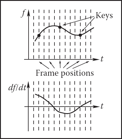
A continuous curve f(t) is fit through the keys provided by the animator even though only values at frame positions are of interest. The derivative of this function gives the speed of parameter change and is at first determined automatically by the fitting procedure.
Most animation systems give the animator the ability to perform interactive fine editing of this initial curve, including inserting more keys, adjusting existing keys, or modifying automatically computed tangents. Another useful technique which can help to tweak the shape of the curve is called TCB control (TCB stands for tension, continuity, and bias). The idea is to introduce three new parameters which can be used to modify the shape of the curve near a key through coordinated adjustment of incoming and outgoing tangents at this point. For keys uniformly spaced in time with distance Δt between them, the standard Catmull-Rom expression for incoming and outgoing tangents at an internal key (tk, fk) can be rewritten as
Modified tangents of a TCB spline are
The tension parameter t controls the sharpness of the curve near the key by scaling both incoming and outgoing tangents. Larger tangents (lower tension) lead to a flatter curve shape near the key. Bias b allows the animator to selectively increase the weight of a key’s neighbors locally pulling the curve closer to a straight line connecting the key with its left (b near 1, “overshooting” the action) or right (b near −1, “undershooting” the action) neighbors. A nonzero value of continuity c makes incoming and outgoing tangents different allowing the animator to create kinks in the curve at the key value. Practically useful values of TCB parameters are typically confined to the interval [−1; 1] with defaults t = c = b = 0 corresponding to the original Catmull-Rom spline. Examples of possible curve shape adjustments are shown in Figure 16.6.

Editing the default interpolating spline (middle column) using TCB controls. Note that all keys remain at the same positions.
16.2.1. Motion Controls
So far, we have described how to control the shape of the animation curve through key positioning and fine tweaking of tangent values at the keys. This, however, is generally not sufficient when one would like to have control both over where the object is moving, i.e., its path, and how fast it moves along this path. Given a set of positions in space as keys, automatic curve-fitting techniques can fit a curve through them, but resulting motion is only constrained by forcing the object to arrive at a specified key position pk at the corresponding key frame tk, and nothing is directly said about the speed of motion between the keys. This can create problems. For example, if an object moves along the x-axis with velocity 11 meters per second for 1 second and then with 1 meter per second for 9 seconds, it will arrive at position x = 20 after 10 seconds thus satisfying animator’s keys (0,0) and (10, 20). It is rather unlikely that this jerky motion was actually desired, and uniform motion with speed 2 meters/second is probably closer to what the animator wanted when setting these keys. Although typically not displaying such extreme behavior, polynomial curves resulting from standard fitting procedures do exhibit nonuniform speed of motion between keys as demonstrated in Figure 16.7. While this can be tolerable (within limits) for some parameters for which the human visual system is not very good at determining nonuniformities in the rate of change (such as color or even rate of rotation), we have to do better for position p of the object where velocity directly corresponds to everyday experience.

All three motions are along the same 2D path and satisfy the set of keys at the tips of the black triangles. The tips of the white triangles show object position at Δt = 1 intervals. Uniform speed of motion between the keys (top) might be closer to what the animator wanted, but automatic fitting procedures could result in either of the other two motions.
We will first distinguish curve parameterization used during the fitting procedure from that used for animation. When a curve is fit through position keys, we will write the result as a function p(u) of some parameter u. This will describe the geometry of the curve in space. The arc length s is the physical length of the curve. A natural way for the animator to control the motion along the now-existing curve is to specify an extra function s(t) which corresponds to how far along the curve the object should be at any given time. To get an actual position in space, we need one more auxiliary function u(s) which computes a parameter value u for given arc length s. The complete process of computing an object position for a given time t is then given by composing these functions (see Figure 16.8):

To get position in space at a given time t, one first utilizes user-specified motion control to obtain the distance along the curve s(t) and then computes the corresponding curve parameter value u(s(t)). Previously fitted curve P(u) can now be used to find the position P(u(s(t))).
Several standard functions can be used as the distance-time function s(t). One of the simplest is the linear function corresponding to constant velocity: s(t) = vt with v = const. Another common example is the motion with constant acceleration a (and initial speed v0) which is described by the parabolic s(t) = v0t + at2/2. Since velocity is changing gradually here, this function can help to model desirable ease-in and ease-out behavior. More generally, the slope of s(t) gives the velocity of motion with negative slope corresponding to the motion backwards along the curve. To achieve most flexibility, the ability to interactively edit s(t) is typically provided to the animator by the animation system. The distance-time function is not the only way to control motion. In some cases it might be more convenient for the user to specify a velocity-time function v(t) or even an acceleration-time function a(t). Since these are correspondingly first and second derivatives of s(t), to use these type of controls, the system first recovers the distance-time function by integrating the user input (twice in the case of a(t)).
The relationship between the curve parameter u and arc length s is established automatically by the system. In practice, the system first determines arc length dependance on parameter u (i.e., the inverse function s(u)). Using this function, for any given S it is possible to solve the equation s(u) − S = 0 with unknown u obtaining u(S). For most curves, the function s(u) cannot be expressed in closed analytic form and numerical integration is necessary (see Chapter 14). Standard numerical root-finding procedures (such as the Newton-Raphson method, for example) can then be directly used to solve the equation s(u) − S = 0 for u.
An alternative technique is to approximate the curve itself as a set of linear segments between points pi computed at some set of sufficiently densely spaced parameter values ui. One then creates a table of approximate arc lengths
Since s(u) is a non-decreasing function of u, one can then find the interval containing the value S by simple searching through the table (see Figure 16.9). Linear interpolation of the interval’s u end values is then performed to finally find u(S). If greater precision is necessary, a few steps of the Newton-Raphson algorithm with this value as the starting point can be applied.

To create a tabular version of s(u), the curve can be approximated by a number of line segments connecting points on the curve positioned at equal parameter increments. The table is searched to find the u-interval for a given S. For the curve above, for example, the value of u corresponding to the position of S = 6.5 lies between u = 0.6 and u = 0.8.
16.2.2 Interpolating Rotation
The techniques presented above can be used to interpolate the keys set for most of the parameters describing the scene. Three-dimensional rotation is one important motion for which more specialized interpolation methods and representations are common. The reason for this is that applying standard techniques to 3D rotations often leads to serious practical problems. Rotation (a change in orientation of an object) is the only motion other than translation which leaves the shape of the object intact. It therefore plays a special role in animating rigid objects.
There are several ways to specify the orientation of an object. First, transformation matrices as described in Chapter 6 can be used. Unfortunately, naive (element-by-element) interpolation of rotation matrices does not produce a correct result. For example, the matrix “halfway” between 2D clock- and counterclockwise 90 degree rotation is the null matrix:
The correct result is, of course, the unit matrix corresponding to no rotation. Second, one can specify arbitrary orientation as a sequence of exactly three rotations around coordinate axes chosen in some specific order. These axes can be fixed in space (fixed-angle representation) or embedded into the object therefore changing after each rotation (Euler-angle representation as shown in Figure 16.10). These three angles of rotation can be animated directly through standard keyframing, but a subtle problem known as gimbal lock arises. Gimbal lock occurs if during rotation one of the three rotation axes is by accident aligned with another, thereby reducing by one the number of available degrees of freedom as shown in Figure 16.11 for a physical device. This effect is more common than one might think—a single 90 degree turn to the right (or left) can potentially put an object into a gimbal lock. Finally, any orientation can be specified by choosing an appropriate axis in space and angle of rotation around this axis. While animating in this representation is relatively straightforward, combining two rotations, i.e., finding the axis and angle corresponding to a sequence of two rotations both represented by axis and angle, is nontrivial. A special mathematical apparatus, quaternions has been developed to make this representation suitable both for combining several rotations into a single one and for animation.

Three Euler angles can be used to specify arbitrary object orientation through a sequence of three rotations around coordinate axes embedded into the object (axis Y always points to the tip of the cone). Note that each rotation is given in a new coordinate system. Fixed angle representation is very similar, but the coordinate axes it uses are fixed in space and do not rotate with the object.

In this example, gimbal lock occurs when a 90 degree turn around axis Z is made. Both X and Y rotations are now performed around the same axis leading to the loss of one degree of freedom.
Given a 3D vector v = (x, y, z) and a scalar s, a quaternion q is formed by combining the two into a four-component object: q = [s x y z] = [s; v]. Several new operations are then defined for quaternions. Quaternion addition simply sums scalar and vector parts separately:
Multiplication by a scalar a gives a new quaternion
More complex quaternion multiplication is defined as
where × denotes a vector cross product. It is easy to see that, similar to matrices, quaternion multiplication is associative, but not commutative. We will be interested mostly in normalized quaternions—those for which the quaternion norm is equal to one. One final definition we need is that of an inverse quaternion:
To represent a rotation by angle ϕ around an axis passing through the origin whose direction is given by the normalized vector n, a normalized quaternion
is formed. To rotate point p, one turns it into the quaternion qp = [0; p] and computes the quaternion product
which is guaranteed to have a zero scalar part and the rotated point as its vector part. Composite rotation is given simply by the product of quaternions representing each of the separate rotation steps. To animate with quaternions, one can treat them as points in a four-dimensional space and set keys directly in this space. To keep quaternions normalized, one should, strictly speaking, restrict interpolation procedures to a unit sphere (a 3D object) in this 4D space. However, a spherical version of even linear interpolation (often called slerp) already results in rather unpleasant math. Simple 4D linear interpolation followed by projection onto the unit sphere shown in Figure 16.12 is much simpler and often sufficient in practice. smoother results can be obtained via repeated application of a linear interpolation procedure using the de Casteljau algorithm.

Interpolating quaternions should be done on the surface of a 3D unit sphere embedded in 4D space. However, much simpler interpolation along a 4D straight line (open circles) followed by reprojection of the results onto the sphere (black circles) is often sufficient.
16.3 Deformations
Although techniques for object deformation might be more properly treated as modeling tools, they are traditionally discussed together with animation methods. Probably the simplest example of an operation which changes object shape is a nonuniform scaling. More generally, some function can be applied to local coordinates of all points specifying the object (i.e., vertices of a triangular mesh or control polygon of a spline surface), repositioning these points and creating a new shape: p′ = f (p, γ) where γ is a vector of parameters used by the deformation function. Choosing different f (and combining them by applying one after another) can help to create very interesting deformations. Examples of useful simple functions include bend, twist, and taper which are shown in Figure 16.13. Animating shape change is very easy in this case by keyframing the parameters of the deformation function. Disadvantages of this technique include difficulty of choosing the mathematical function for some nonstandard deformations and the fact that the resulting deformation is global in the sense that the complete object, and not just some part of it, is reshaped.
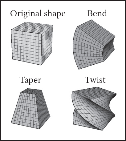
Popular examples of global deformations. Bending and twist angles, as well as the degree of taper, can all be animated to achieve dynamic shape change.
To deform an object locally while providing more direct control over the result, one can choose a single vertex, move it to a new location and adjust vertices within some neighborhood to follow the seed vertex. The area affected by the deformation and the specific amount of displacement in different parts of the object are controlled by an attenuation function which decreases with distance (typically computed over the object’s surface) to the seed vertex. Seed vertex motion can be keyframed to produce animated shape change.
A more general deformation technique is called free-form deformation (FFD) (Sederberg & Parry, 1986). A local (in most cases rectilinear) coordinate grid is first established to encapsulate the part of the object to be deformed, and coordinates (s, t, u) of all relevant points are computed with respect to this grid. The user then freely reshapes the grid of lattice points Pijk into a new distorted lattice (Figure 16.14). The object is reconstructed using coordinates computed in the original undistorted grid in the trivariate analog of Bézier interpolants (see Chapter 15) with distorted lattice points serving as control points in this expression:

where L, M, N are maximum indices of lattice points in each dimension. In effect, the lattice serves as a low-resolution version of the object for the purpose of deformation, allowing for a smooth shape change of an arbitrarily complex object through a relatively small number of intuitive adjustments. FFD lattices can themselves be treated as regular objects by the system and can be transformed, animated, and even further deformed if necessary, leading to corresponding changes in the object to which the lattice is attached. For example, moving a deformation tool consisting of the original lattice and distorted lattice representing a bulge across an object results in a bulge moving across the object.
16.4 Character Animation
Animation of articulated figures is most often performed through a combination of keyframing and specialized deformation techniques. The character model intended for animation typically consists of at least two main layers as shown in Figure 16.15. The motion of a highly detailed surface representing the outer shell or skin of the character is what the viewer will eventually see in the final product. The skeleton underneath it is a hierarchical structure (a tree) of joints which provides a kinematic model of the figure and is used exclusively for animation. In some cases, additional intermediate layer(s) roughly corresponding to muscles are inserted between the skeleton and the skin.

(Left) A hierarchy of joints, a skeleton, serves as a kinematic abstraction of the character; (middle) repositioning the skeleton deforms a separate skin object attached to it; (right) a tree data structure is used to represent the skeleton. For compactness, the internal structure of several nodes is hidden (they are identical to a corresponding sibling).
Each of the skeleton’s joints acts as a parent for the hierarchy below it. The root represents the whole character and is positioned directly in the world coordinate system. If a local transformation matrix which relates a joint to its parent in the hierarchy is available, one can obtain a transformation which relates local space of any joint to the world system (i.e., the system of the root) by simply concatenating transformations along the path from the root to the joint. To evaluate the whole skeleton (i.e., find position and orientation of all joints), a depth-first traversal of the complete tree of joints is performed. A transformation stack is a natural data structure to help with this task. While traversing down the tree, the current composite matrix is pushed on the stack and a new one is created by multiplying the current matrix with the one stored at the joint. When backtracking to the parent, this extra transformation should be undone before another branch is visited; this is easily done by simply popping the stack. Although this general and simple technique for evaluating hierarchies is used throughout computer graphics, in animation (and robotics) it is given a special name—forward kinematics (FK). While general representations for all transformations can be used, it is common to use specialized sets of parameters, such as link lengths or joint angles, to specify skeletons. To animate with forward kinematics, rotational parameters of all joints are manipulated directly. The technique also allows the animator to change the distance between joints (link lengths), but one should be aware that this corresponds to limb stretching and can often look rather unnatural.
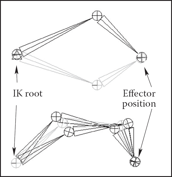
Forward kinematics requires the user to set parameters for all joints involved in the motion (Figure 16.16 (top)). Most of these joints, however, belong to internal nodes of the hierarchy, and their motion is typically not something the animator wants to worry about. In most situations, the animator just wants them to move naturally “on their own,” and one is much more interested in specifying the behavior of the endpoint of a joint chain, which typically corresponds to something performing a specific action, such as an ankle or a tip of a finger. The animator would rather have parameters of all internal joints be determined from the motion of the end effector automatically by the system. Inverse kinematics (IK) allows us to do just that (see Figure 16.16 (bottom)).

Forward kinematics (top) requires the animator to put all joints into correct position. In inverse kinematic (bottom), parameters of some internal joints are computed based on desired end effector motion.
Let x be the position of the end effector and α be the vector of parameters needed to specify all internal joints along the chain from the root to the final joint. Sometimes the orientation of the final joint is also directly set by the animator, in which case we assume that the corresponding variables are included in the vector x. For simplicity, however, we will write all specific expressions for the vector:
Since each of the variables in x is a function of α, it can be written as a vector equation x = F(α). If we change the internal joint parameters by a small amount δα, a resulting change δx in the position of the end effector can be approximately written as
where is the matrix of partial derivatives called the Jacobian:
At each moment in time, we know the desired position of the end effector (set by the animator) and, of course, the effector’s current position. Subtracting the two, we will get the desired adjustment δx. Elements of the Jacobian matrix are related to changes in a coordinate of the end effector when a particular internal parameter is changed while others remain fixed (see Figure 16.17). These elements can be computed for any given skeleton configuration using geometric relationships. The only remaining unknowns in the system of equations (16.1) are the changes in internal parameters α. Once we solve for them, we update α = α+δα which gives all the necessary information for the FK procedure to reposition the skeleton.

Partial derivative ∂x/∂αknee is given by the limit of Δx/Δαknee. Effector displacement is computed while all joints, except the knee, are kept fixed.
Unfortunately, the system (16.1) cannot usually be solved analytically and, moreover, it is in most cases underconstrained, i.e., the number of unknown internal joint parameters α exceeds the number of variables in vector x. This means that different motions of the skeleton can result in the same motion of the end effector. Some examples are shown on Figure 16.18. Many ways of obtaining specific solution for such systems are available, including those taking into account natural constraints needed for some real-life joints (bending a knee only in one direction, for example). One should also remember that the computed Jacobian matrix is valid only for one specific configuration, and it has to be updated as the skeleton moves. The complete IK framework is presented in Figure 16.19. Of course, the root joint for IK does not have to be the root of the whole hierarchy, and multiple IK solvers can be applied to independent parts of the skeleton. For example, one can use separate solvers for right and left feet and yet another one to help animate grasping with the right hand, each with its own root.
Multiple configurations of internal joints can result in the same effector position. (Top) disjoint “flipped” solutions; (bottom) a continuum of solutions.

A combination of FK and IK approaches is typically used to animate the skeleton. Many common motions (walking or running cycles, grasping, reaching, etc.) exhibit well-known patterns of mutual joint motion making it possible to quickly create naturally looking motion or even use a library of such “clips.” The animator then adjusts this generic result according to the physical parameters of the character and also to give it more individuality.
When a skeleton changes its position, it acts as a special type of deformer applied to the skin of the character. The motion is transferred to this surface by assigning each skin vertex one (rigid skinning) or more (smooth skinning) joints as drivers (see Figure 16.20). In the first case, a skin vertex is simply frozen into the local space of the corresponding joint, which can be the one nearest in space or one chosen directly by the user. The vertex then repeats whatever motion this joint experiences, and its position in world coordinates is determined by standard FK procedure. Although it is simple, rigid skinning makes it difficult to obtain sufficiently smooth skin deformation in areas near the joints or also for more subtle effects resembling breathing or muscle action. Additional specialized deformers called flexors can be used for this purpose. In smooth skinning, several joints can influence a skin vertex according to some weight assigned by the animator, providing more detailed control over the results. Displacement vectors, di, suggested by different joints affecting a given skin vertex (each again computed with standard FK) are averaged according to their weights wi to compute the final displacement of the vertex d = Σ widi. Normalized weights (Σwi = 1) are the most common but not fundamentally necessary. Setting smooth skinning weights to achieve the desired effect is not easy and requires significant skill from the animator.
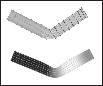
Top: Rigid skinning assigns skin vertices to a specific joint. Those belonging to the elbow joint are shown in black; Bottom: Soft skinning can blend the influence of several joints. Weights for the elbow joint are shown (lighter = greater weight). Note smoother skin deformation of the inner part of the skin near the joint.
16.4.1 Facial Animation
Skeletons are well suited for creating most motions of a character’s body, but they are not very convenient for realistic facial animation. The reason is that the skin of a human face is moved by muscles directly attached to it, contrary to other parts of the body where the primary objective of the muscles is to move the bones of the skeleton and any skin deformation is a secondary outcome. The result of this facial anatomical arrangement is a very rich set of dynamic facial expressions humans use as one of the main instruments of communication. We are all very well trained to recognize such facial variations and can easily notice any unnatural appearance. This not only puts special demands on the animator but also requires a high-resolution geometric model of the face and, if photorealism is desired, accurate skin reflection properties and textures.
While it is possible to set key poses of the face vertex-by-vertex and interpolate between them or directly simulate the behavior of the underlying muscle structure using physics-based techniques (see Section 16.5), more specialized high-level approaches also exist. The static shape of a specific face can be characterized by a relatively small set of so-called conformational parameters (overall scale, distance from the eye to the forehead, length of the nose, width of the jaws, etc.) which are used to morph a generic face model into one with individual features. An additional set of expressive parameters can be used to describe the dynamic shape of the face for animation. Examples include rigid rotation of the head, how wide the eyes are open, movement of some feature point from its static position, etc. These are chosen so that most of the interesting expressions can be obtained through some combination of parameter adjustments, therefore, allowing a face to be animated via standard keyframing. To achieve a higher level of control, one can use expressive parameters to create a set of expressions corresponding to common emotions (neutral, sadness, happiness, anger, surprise, etc.) and then blend these key poses to obtain a “slightly sad” or “angrily surprised” face. Similar techniques can be used to perform lip-synch animation, but key poses in this case correspond to different phonemes. Instead of using a sequence of static expressions to describe a dynamic one, the Facial Action Coding System (FACS) (Eckman & Friesen, 1978) decomposes dynamic facial expressions directly into a sum of elementary motions called action units (AUs). The set of AUs is based on extensive psychological research and includes such movements as raising the inner brow, wrinkling the nose, stretching lips, etc. Combining AUs can be used to synthesize a necessary expression.
16.4.2 Motion Capture
Even with the help of the techniques described above, creating realistic-looking character animation from scratch remains a daunting task. It is therefore only natural that much attention is directed toward techniques which record an actor’s motion in the real world and then apply it to computer-generated characters. Two main classes of such motion capture (MC) techniques exist: electromagnetic and optical.
In electromagnetic motion capture, an electromagnetic sensor directly measures its position (and possibly orientation) in 3D, often providing the captured results in real time. Disadvantages of this technique include significant equipment cost, possible interference from nearby metal objects, and noticeable size of sensors and batteries which can be an obstacle in performing high-amplitude motions. In optical MC, small colored markers are used instead of active sensors making it a much less intrusive procedure. Figure 16.21 shows the operation of such a system. In the most basic arrangement, the motion is recorded by two calibrated video cameras, and simple triangulation is used to extract the marker’s 3D position. More advanced computer vision algorithms used for accurate tracking of multiple markers from video are computationally expensive, so, in most cases, such processing is done offline. Optical tracking is generally less robust than electromagnetic. Occlusion of a given marker in some frames, possible misidentification of markers, and noise in images are just a few of the common problem which have to be addressed. Introducing more cameras observing the motion from different directions improves both accuracy and robustness, but this approach is more expensive and it takes longer to process such data. Optical MC becomes more attractive as available computational power increases and better computer vision algorithms are developed. Because of low impact nature of markers, optical methods are suitable for delicate facial motion capture and can also be used with objects other than humans—for example, animals or even tree branches in the wind.

Optical motion capture: markers attached to a performer’s body allow skeletal motion to be extracted.
Image courtesy of Motion Analysis Corp.
With several sensors or markers attached to a performer’s body, a set of time-dependant 3D positions of some collection of points can be recorded. These tracking locations are commonly chosen near joints, but, of course, they still lie on skin surface and not at points where actual bones meet. Therefore, some additional care and a bit of extra processing is necessary to convert recorded positions into those of the physical skeleton joints. For example, putting two markers on opposite sides of the elbow or ankle allows the system to obtain better joint position by averaging locations of the two markers. Without such extra care, very noticeable artifacts can appear due to offset joint positions as well as inherent noise and insufficient measurement accuracy. Because of physical inaccuracy during motion, for example, character limbs can lose contact with objects they are supposed to touch during walking or grasping, problems like foot-sliding (skating) of the skeleton can occur. Most of these problems can be corrected by using inverse kinematics techniques which can explicitly force the required behavior of the limb’s end.
Recovered joint positions can now be directly applied to the skeleton of a computer-generated character. This procedure assumes that the physical dimensions of the character are identical to those of the performer. Retargeting recorded motion to a different character and, more generally, editing MC data, requires significant care to satisfy necessary constraints (such as maintaining feet on the ground or not allowing an elbow to bend backwards) and preserve an overall natural appearance of the modified motion. Generally, the greater the desired change from the original, the less likely it will be possible to maintain the quality of the result. An interesting approach to the problem is to record a large collection of motions and stitch together short clips from this library to obtain desired movement. Although this topic is currently a very active research area, limited ability to adjust the recorded motion to the animator’s needs remains one of the main disadvantages of motion capture technique.
16.5 Physics-Based Animation
The world around us is governed by physical laws, many of which can be formalized as sets of partial or, in some simpler cases, ordinary differential equations. One of the original applications of computers was (and remains) solving such equations. It is therefore only natural to attempt to use numerical techniques developed over the several past decades to obtain realistic motion for computer animation.
Because of its relative complexity and significant cost, physics-based animation is most commonly used in situations when other techniques are either unavailable or do not produce sufficiently realistic results. Prime examples include animation of fluids (which includes many gaseous phase phenomena described by the same equations—smoke, clouds, fire, etc.), cloth simulation (an example is shown in Figure 16.22), rigid body motion, and accurate deformation of elastic objects. Governing equations and details of commonly used numerical approaches are different in each of these cases, but many fundamental ideas and difficulties remain applicable across applications. Many methods for numerically solving ODEs and PDEs exist, but discussing them in details is far beyond the scope of this book. To give the reader a flavor of physics-based techniques and some of the issues involved, we will briefly mention here only the finite difference approach—one of the conceptually simplest and most popular families of algorithms which has been applied to most, if not all, differential equations encountered in animation.

Realistic cloth simulation is often performed with physics-based methods. In this example, forces are due to collisions and gravity.
The key idea of this approach is to replace a differential equation with its discrete analog—a difference equation. To do this, the continuous domain of interest is represented by a finite set of points at which the solution will be computed. In the simplest case, these are defined on a uniform rectangular grid as shown in Figure 16.23. Every derivative present in the original ODE or PDE is then replaced by its approximation through function values at grid points. One way of doing this is to subtract the function value at a given point from the function value for its neighboring point on the grid:
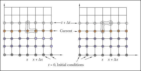
Two possible difference schemes for an equation involving derivatives ∂f/∂x and ∂f/∂t. (Left) An explicit scheme expresses unknown values (open circles) only through known values at the current (orange circles) and possibly past (blue circles) time; (Right) Implicit schemes mix known and unknown values in a single equation making it necessary to solve all such equations as a system. For both schemes, information about values on the right boundary is needed to close the process.
These expressions are, of course, not the only way. One can, for example, use f(t − Δt) instead of f(t) above and divide by 2Δt. For an equation containing a time derivative, it is now possible to propagate values of an unknown function forward in time in a sequence of Δt-size steps by solving the system of difference equations (one at each spatial location) for unknown f(t + Δt). Some initial conditions, i.e., values of the unknown function at t = 0, are necessary to start the process. Other information, such as values on the boundary of the domain, might also be required depending on the specific problem.
The computation of f(t+Δt) can be done easily for so-called explicit schemes when all other values present are taken at the current time and the only unknown in the corresponding difference equation f(t + Δt) is expressed through these known values. Implicit schemes mix values at current and future times and might use, for example,
as an approximation of . In this case one has to solve a system of algebraic equations at each step.
The choice of difference scheme can dramatically affect all aspects of the algorithm. The most obvious among them is accuracy. In the limit Δt → 0 or Δx → 0, expressions of the type in Equation (16.2) are exact, but for finite step size some schemes allow better approximation of the derivative than others. Stability of a difference scheme is related to how fast numerical errors, which are always present in practice, can grow with time. For stable schemes this growth is bounded, while for unstable ones it is exponential and can quickly overwhelm the solution one seeks (see Figure 16.24). It is important to realize that while some inaccuracy in the solution is tolerable (and, in fact, accuracy demanded in physics and engineering is rarely needed for animation), an unstable result is completely meaningless, and one should avoid using unstable schemes. Generally, explicit schemes are either unstable or can become unstable at larger step sizes while implicit ones are unconditionally stable. Implicit schemes allows greater step size (and, therefore, fewer steps) which is why they are popular despite the need to solve a system of algebraic equations at each step. Explicit schemes are attractive because of their simplicity if their stability conditions can be satisfied. Developing a good difference scheme and corresponding algorithm for a specific problem is not easy, and for most standard situations it is well advised to use an existing method. Ample literature discussing details of these techniques is available.

An unstable solution might follow the exact one initially, but can deviate arbitrarily far from it with time. Accuracy of a stable solution might still be insufficient for a specific application.
One should remember that, in many cases, just computing all necessary terms in the equation is a difficult and time-consuming task on its own. In rigid body or cloth simulation, for example, most of the forces acting on the system are due to collisions among objects. At each step during animation, one therefore has to solve a purely geometric, but very nontrivial, problem of collision detection. In such conditions, schemes which require fewer evaluations of such forces might provide significant computational savings.
Although the result of solving appropriate time-dependant equations gives very realistic motion, this approach has its limitations. First of all, it is very hard to control the result of physics-based animation. Fundamental mathematical properties of these equations state that once the initial conditions are set, the solution is uniquely defined. This does not leave much room for animator input and, if the result is not satisfactory for some reason, one has only a few options. They are mostly limited to adjusting initial condition used, changing physical properties of the system, or even modifying the equations themselves by introducing artificial terms intended to “drive” the solution in the direction the animator wants. Making such changes requires significant skill as well as understanding of the underlying physics and, ideally, numerical methods. Without this knowledge, the realism provided by physics-based animation can be destroyed or severe numerical problems might appear.
16.6 Procedural Techniques
Imagine that one could write (and implement on a computer) a mathematical function which outputs precisely the desired motion given some animator guidance. Physics-based techniques outlined above can be treated as a special case of such an approach when the “function” involved is the procedure to solve a particular differential equation and “guidance” is the set of initial and boundary conditions, extra equation terms, etc.
However, if we are only concerned with the final result, we do not have to follow a physics-based approach. For example, a simple constant amplitude wave on the surface of a lake can be directly created by applying the function f(x, t) = A cos(ωt - kx + ϕ) with constant frequency ω, wave vector k and phase ϕ to get displacement at the 2D point x at time t. A collection of such waves with random phases and appropriately chosen amplitudes, frequencies, and wave vectors can result in a very realistic animation of the surface of water without explicitly solving any fluid dynamics equations. It turns out that other rather simple mathematical functions can also create very interesting patterns or objects. Several such functions, most based on lattice noises, have been described in Section 11.5. Adding time dependance to these functions allows us to animate certain complex phenomena much easier and cheaper than with physics-based techniques while maintaining very high visual quality of the results. If noise(x) is the underlying pattern-generating function, one can create a time-dependant variant of it by moving the argument position through the lattice. The simplest case is motion with constant speed: timenoise(x, t) = noise(x + vt), but more complex motion through the lattice is, of course, also possible and, in fact, more common. One such path, a spiral, is shown in Figure 16.25. Another approach is to animate parameters used to generate the noise function. This is especially appropriate if the appearance changes significantly with time—a cloud becoming more turbulent, for example. In this way one can animate the dynamic process of formation of clouds using the function which generates static ones.

A path through the cube defining procedural noise is traversed to animate the resulting pattern.
For some procedural techniques, time dependance is a more integral component. The simplest cellular automata operate on a 2D rectangular grid where a binary value is stored at each location (cell). To create a time varying pattern, some user-provided rules for modifying these values are repeatedly applied. Rules typically involve some set of conditions on the current value and that of the cell’s neighbors. For example, the rules of the popular 2D Game of Life cellular automaton invented in 1970 by British mathematician John Conway are the following:
- A dead cell (i.e., binary value at a given location is 0) with exactly three live neighbors becomes a live cell (i.e., its value set to 1).
- A live cell with two or three live neighbors stays alive.
- In all other cases, a cell dies or remains dead.
Once the rules are applied to all grid locations, a new pattern is created and a new evolution cycle can be started. Three sample snapshots of the live cell distribution at different times are shown in Figure 16.26. More sophisticated automata simultaneously operate on several 3D grids of possibly floating point values and can be used for modeling dynamics of clouds and other gaseous phenomena or biological systems for which this apparatus was originally invented (note the terminology). Surprising pattern complexity can arise from just a few well-chosen rules, but how to write such rules to create the desired behavior is often not obvious. This is a common problem with procedural techniques: there is only limited, if any, guidance on how to create new procedures or even adjust parameters of existing ones. Therefore, a lot of tweaking and learning by trial-and-error (“by experience”) is usually needed to unlock the full potential of procedural methods.

Several (non-consecutive) stages in the evolution of a Game of Life automaton. Live cells are shown in black. Stable objects, oscillators, traveling patterns, and many other interesting constructions can result from the application of very simple rules.
Figure created using a program by Alan Hensel.
Another interesting approach which was also originally developed to describe biological objects is the technique called L-systems (after the name of their original inventor, Astrid Lindenmayer). This approach is based on grammars or sets of recursive rules for rewriting strings of symbols. There are two types of symbols: terminal symbols stand for elements of something we want to represent with a grammar. Depending on their meaning, grammars can describe structure of trees and bushes, buildings and whole cities, or programming and natural languages. In animation, L-systems are most popular for representing plants and corresponding terminals are instructions to the geometric modeling system: put a leaf (or a branch) at a current position—we will use the symbol @ and just draw a circle, move current position forward by some number of units (symbol f), turn current direction 60 degrees around world Z-axis (symbol +), pop (symbol [) or push (symbol]) current position/orientation, etc. Auxiliary nonterminal symbols (denoted by capital letters) have only semantic rather than any direct meaning. They are intended to be eventually rewritten through terminals. We start from the special nonterminal start symbol S and keep applying grammar rules to the current string in parallel, i.e., replace all nonterminals currently present to get the new string, until we end up with a string containing only terminals and no more substitution is therefore possible. This string of modeling instructions is then used to output the actual geometry. For example, a set of rules (productions)
might result in the following sequence of rewriting steps demonstrated in Figure 16.27:

Consecutive derivation steps using a simple L-system. Capital letters denote nonterminals and illustrate positions at which corresponding nonterminal will be expanded. They are not part of the actual output.
As shown above, there are typically many different productions for the same nonterminal allowing the generation of many different objects with the same grammar. The choice of which rule to apply can depend on which symbols are located next to the one being replaced (context-sensitivity) or can be performed at random with some assigned probability for each rule (stochastic L-systems). More complex rules can model interaction with the environment, such as pruning to a particular shape, and parameters can be associated with symbols to control geometric commands issued.
L-systems already capture plant topology changes with time: each intermediate string obtained in the rewriting process can be interpreted as a “younger” version of the plant (see Figure 16.27). For more significant changes, different productions can be in effect at different times allowing the structure of the plant to change significantly as it grows. A young tree, for example, produces a lot of new branches, while an older one branches only moderately.
Very realistic plant models have been created with L-systems. However, as with most procedural techniques, one needs some experience to meaningfully apply existing L-systems, and writing new grammars to capture some desired effect is certainly not easy.
16.7 Groups of Objects
To animate multiple objects one can, of course, simply apply standard techniques described in the chapter so far to each of them. This works reasonably well for a moderate number of independent objects whose desired motion is known in advance. However, in many cases, some kind of coordinated action in a dynamic environment is necessary. If only a few objects are involved, the animator can use an artificial intelligence (AI)-based system to automatically determine immediate tasks for each object based on some high-level goal, plan necessary motion, and execute the plan. Many modern games use such autonomous objects to create smart monsters or player’s collaborators.
Interestingly, as the number of objects in a group grows from just a few to several dozens, hundreds, and thousands, individual members of a group must have only very limited “intelligence” in order for the group as a whole to exhibit what looks like coordinated goal-driven motion. It turns out that this flocking is emergent behavior which can arise as a result of limited interaction of group members with just a few of their closest neighbors (Reynolds, 1987). Flocking should be familiar to anyone who has observed the fascinatingly synchronized motion of a flock of birds or a school of fish. The technique can also be used to control groups of animals moving over terrain or even a human crowd.
At any given moment, the motion of a member of a group, often called boid when applied to flocks, is the result of balancing several often contradictory tendencies, each of which suggests its own velocity vector (see Figure 16.28). First, there are external physical forces F acting on the boid, such as gravity or wind. New velocity due to those forces can be computed directly through Newton’s law as
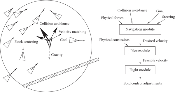
(Left) Individual flock member (boid) can experience several urges of different importance (shown by line thickness) which have to be negotiated into a single velocity vector. A boid is aware of only its limited neighborhood (circle). (Right) Boid control is commonly implemented as three separate modules.
Second, a boid should react to global environment and to the behavior of other group members. Collision avoidance is one of the main results of such interaction. It is crucial for flocking that each group member has only limited field of view, and therefore is aware only of things happening within some neighborhood of its current position. To avoid objects in the environment, the simplest, if imperfect, strategy is to set up a limited extent repulsive force field around each such object. This will create a second desired velocity vector , also given by Newton’s law. Interaction with other group members can be modeled by simultaneously applying different steering behaviors resulting in several additional desired velocity vectors . Moving away from neighbors to avoid crowding, steering toward flock mates to ensure flock cohesion, and adjusting a boid’s speed to align with average heading of neighbors are most common. Finally, some additional desired velocity vectors are usually applied to achieve needed global goals. These can be vectors along some path in space, following some specific designated leader of the flock, or simply representing migratory urge of a flock member.
Once all vnew are determined, the final desired vector is negotiated based on priorities among them. Collision avoidance and velocity matching typically have higher priority. Instead of simple averaging of desired velocity vectors which can lead to cancellation of urges and unnatural “moving nowhere” behavior, an acceleration allocation strategy is used. Some fixed total amount of acceleration is made available for a boid and fractions of it are being given to each urge in order of priority. If the total available acceleration runs out, some lower priority urges will have less effect on the motion or be completely ignored. The hope is that once the currently most important task (collision avoidance in most situations) is accomplished, other tasks can be taken care of in near future. It is also important to respect some physical limitations of real objects, for example, clamping too high accelerations or speeds to some realistic values. Depending on the internal complexity of the flock member, the final stage of animation might be to turn the negotiated velocity vector into a specific set of parameters (bird’s wing positions, orientation of plane model in space, leg skeleton bone configuration) used to control a boid’s motion. A diagram of a system implementing flocking is shown on Figure 16.28 (right).
A much simpler, but still very useful, version of group control is implemented by particle systems (Reeves, 1983). The number of particles in a system is typically much larger than number of boids in a flock and can be in the tens or hundreds of thousands, or even more. Moreover, the exact number of particles can fluctuate during animation with new particles being born and some of the old ones destroyed at each step. Particles are typically completely independent from each other, ignoring one’s neighbors and interacting with the environment only by experiencing external forces and collisions with objects, not through collision avoidance as was the case for flocks. At each step during animation, the system first creates new particles with some initial parameters, terminates old ones, and then computes necessary forces and updates velocities and positions of the remaining particles according to Newton’s law.

After being emitted by a directional source, particles collide with an object and then are blown down by a local wind field once they clear the obstacle.
All parameters of a particle system (number of particles, particle life span, initial velocity, and location of a particle, etc.) are usually under the direct control of the animator. Prime applications of particle systems include modeling fireworks, explosions, spraying liquids, smoke and fire, or other fuzzy objects and phenomena with no sharp boundaries. To achieve a realistic appearance, it is important to introduce some randomness to all parameters, for example, having a random number of particles born (and destroyed) at each step with their velocities generated according to some distribution. In addition to setting appropriate initial parameters, controlling the motion of a particle system is commonly done by creating a specific force pattern in space—blowing a particle in a new direction once it reaches some specific location or adding a center of attraction, for example. One should remember that with all their advantages, simplicity of implementation and ease of control being the prime ones, particle systems typically do not provide the level of realism characteristic of true physics-based simulation of the same phenomena.
Notes
In this chapter we have concentrated on techniques used in 3D animation. There also exist a rich set of algorithms to help with 2D animation production and post-processing of images created by computer graphics rendering systems. These include techniques for cleaning up scanned-in artist drawings, feature extraction, automatic 2D in-betweening, colorization, image warping, enhancement and compositing, and many others.
One of the most significant developments in the area of computer animation has been the increasing power and availability of sophisticated animation systems. While different in their specific set of features, internal structure, details of user interface, and price, most such systems include extensive support not only for animation, but also for modeling and rendering, turning them into complete production platforms. It is also common to use these systems to create still images. For example, many images for figures in this section were produced using Maya software generously donated by Alias.
Large-scale animation production is an extremely complex process which typically involves a combined effort by dozens of people with different backgrounds spread across many departments or even companies. To better coordinate this activity, a certain production pipeline is established which starts with a story and character sketches, proceeds to record necessary sound, build models, and rig characters for animation. Once actual animation commences, it is common to go back and revise the original designs, models, and rigs to fix any discovered motion and appearance problems. Setting up lighting and material properties is then necessary, after which it is possible to start rendering. In most sufficiently complex projects, extensive postprocessing and compositing stages bring together images from different sources and finalize the product.
We conclude this chapter by reminding the reader that in the field of computer animation, any technical sophistication is secondary to a good story, expressive characters, and other artistic factors, most of which are hard or simply impossible to quantify. It is safe to say that Snow White and her seven dwarfs will always share the screen with green ogres and donkeys, and most of the audience will be much more interested in the characters and the story rather than in which, if any, computers (and in what exact way) helped to create them.