
Now that you have an understanding of how to use the Audacity 2 Effect menu to implement algorithmic effects and plug-in filter processing in your digital audio editing, it is time to look at how you should visualize the digital audio frequencies that comprise your data sample waveforms.
In this chapter, you’ll look at how to visualize waveform frequency distribution using Audacity’s Analyze menu, along with the Plot Spectrum feature, so that you can see exactly what you are doing before and after your digital audio editing “moves,” such as the algorithmic processing that you’ve done in the past several chapters.
You’ll look at all the different types of analysis that Audacity can do, including its spectrum analysis features.
Audacity Analyze Menu: Sample Analysis
Audacity’s effects and filters aren’t the only tools that utilize algorithms; there are also a number of useful audio data analysis tools that use algorithms, which are configured using front-end dialogs, just like the effects and filters featured in Chapters 5–8. There are tools in Audacity’s Analyze menu
(yes, analysis has its own menu) for contrast (volume) analysis between audio selections, clipping analysis, finding beats, creating label track labels, exporting sample data analysis, and locating silence and the opposite of silence, which are sound samples.
You’ll explore several of the most useful tools in the Analyze menu and build on this knowledge in the next few chapters. You’ll learn how to generate a label track and conform it to vocal samples, how to export sample analysis, and how to do spectral analysis.
Regular Interval Labels: Automatic Sample Labels
Click the Analyze menu at the top right of the Audacity menuing system and look at the eight analysis tools available to do tedious digital audio analysis chores. Select the Regular Interval Labels and let Audacity create a label track and insert labels for your vocal subsamples.
The Regular Interval Labels dialog is shown in Figure 9-1; it allows you to automate a subsample labeling process. Place your first label at 0.0 [seconds]. In the Label placement method drop-down menu, use the Number of labels option (set it at 4). Set the Label text to vocal. Set the Minimum number of digits to None. Set a Yes value for both Add final label and Adjust label interval to fit length, and then click on OK.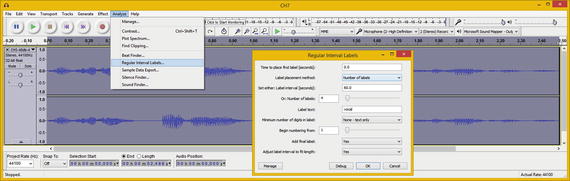
Figure 9-1.
Audacity Analyze menu and Regular Interval Labels
As you can see in Figure 9-2, Audacity created label data in a Label Track underneath the Stereo Track, and labeled each vocal using a generic name, vocal, and left a data field ready to edit in the first (leftmost) data field, as shown in white at the bottom left of the screenshot. Backspace over the word vocal and type Digital to rename this first label.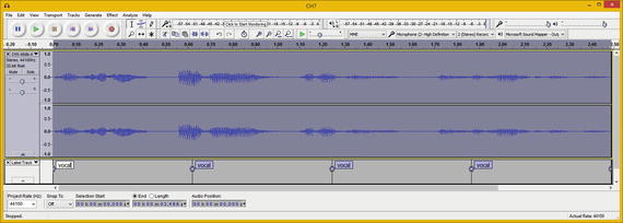
Figure 9-2.
Regular Interval Labels in their own Audacity track
You can also place your mouse cursor over the dots on the lines that separate these labels, and when they turn white, as shown in the Fundamentals label, click and drag to position the lines where the audio subsamples begin and end, as I have done.
As you can see in Figure 9-3, once you name and position all of the label indicators, you have a great guide for your project, so that others can see what the sample data relates to.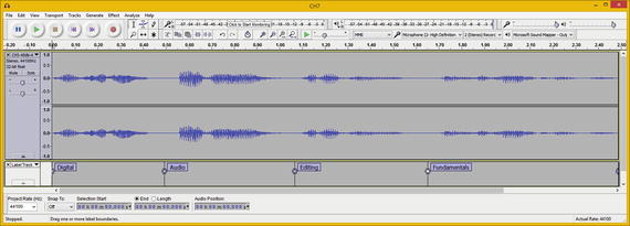
Figure 9-3.
Name and Position label indicators for each sample
Not only can you drag the dots, which position the lines and arrowheads, but you can also drag each directional arrowhead to define the exact range of the subsample area. I have done this in Figure 9-4 so that you can see how these labels center their text label portions (or try, at least) once you fine-tune their range using the < and > arrowhead icons at the end of each label range in the Label Track.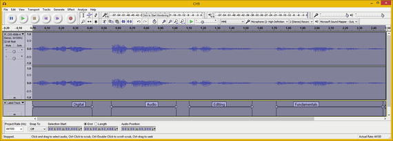
Figure 9-4.
Use label arrowheads, to show sample waveform spans
Next, let’s look at Sample Data Export, an Analysis menu function that exports sample data analysis based on the parameters that you give the algorithm.
Sample Data Export: Export Sample Data Analysis
Select the Analyze drop-down menu and then select the Sample Data Export option (see Figure 9-5). This opens the Sample Data Export dialog, where you can specify the number of samples, the measurement scale, the file data format, the header information to include in the file, the header text, the stereo channel data layout, the file name, the output folder, and the options to show messages and overwrite the data analysis files.
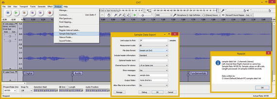
Figure 9-5.
Audacity Analyze menu and Sample Data Export dialog
I decided to generate 24 data samples using decibels in a Sample List text data format that could be parsed (processed) with code (Java, JavaScript, etc.). I used Standard header information and displayed stereo sample analysis data on the same line. I set Show messages to Yes and Allow files to be overwritten to No. I named the file sample-data and used the default Home directory output folder, which for Windows is the Users folder.
Click the OK button to generate the sample data analysis in your Users folder in the sample-data.txt file. I took a screenshot (see Figure 9-6) of my Windows Explorer file management utility, which shows the C:UsersDefault.Default.PC folder for my workstation and a sample-data.txt analysis file.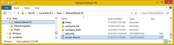
Figure 9-6.
Find your sample-data.txt file in your Users folder
I right-clicked the sample-data.txt file and selected the Open with Notepad (the Windows text editor) option to review the sample analysis data (see Figure 9-7). As you can see in line 18 of the file, there is a decibel spike of 90 for the right channel, where your decibel level is almost twice the normal 45. This is the type of data visualization that the tool provides, along with sample analysis data that can be used in advanced ways in your programming applications.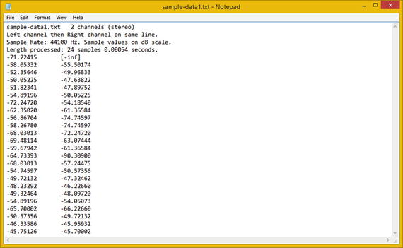
Figure 9-7.
View your sample-data.txt file in your text editor
Next, let’s look at how you can visualize an audio frequency spectrum that exists inside the audio data sample.
Frequency Spectrum Data Analysis Tools
As you have seen in this book thus far, it can be very difficult to do digital audio editing techniques using only your ears, unless you’re one of those few people who have exceptional hearing abilities. For this reason, I have showed you tools or work processes that allow you to visualize sample editing data using file size data, waveforms, and sample data analysis tools. The next Audacity data visualization tool that you are going to learn about is exceptionally powerful, as it allows you to create and view a graph representation of a sample frequency spectrum.
Spectral Analysis: Audacity’s Plot Spectrum Dialog
There is a
Plot Spectrum tool
in the Analyze menu that allows you to see the frequency spectrum using algorithm and frequency sampling resolution options. I recommend that you spend some time playing with the Analyze ➤ Plot Spectrum function (shown in Figure 9-8) on your own as well, after going through some of the options presented in this chapter.
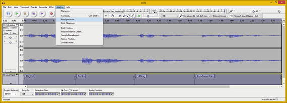
Figure 9-8.
Select the Analyze ➤ Plot Spectrum menu sequence
As you can see in Figure 9-9, the first thing that I did was visualize the Notch Filter
(that you used in Chapter 8) to see if it looks as if I took a notch out of the data sample. As you can clearly see in the right-hand screenshot, there is indeed a clear notch at 4500 Hz. You’ll take a look at some of these other settings as well.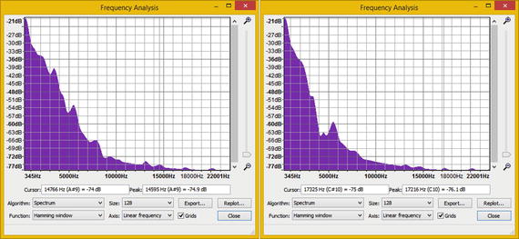
Figure 9-9.
Spectrum Algorithm Size 128, pre/post Notch Filter
The first thing that you’ll look at is how to set the frequency display resolution by using the Frequency Analysis’s Size drop-down menu. I set it to 256 in the “before” and “after” data samples, so that you can see how it adds more peak data, as the two dialogs show you in Figure 9-10. I’ll also show you 512 and 1024 settings later on, so that you can see how these settings visualize your spectrum data.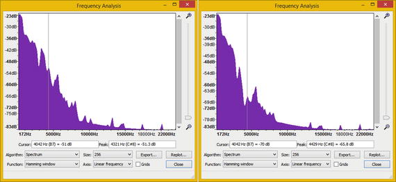
Figure 9-10.
Spectrum Algorithm Size 256, pre/post Notch Filter
What you have looked at so far is a spectral analysis for your entire data sample; but as you may have surmised, you can also use this tool to analyze subsamples. Let’s take a look at that next, as this is an even more useful analysis approach.
Subsample Analysis: Using the Select Tool
Let’s select the vocal for Audio, as shown in Figure 9-11. This is made clearer since adding your handy Label Track and the custom label markers that you installed earlier in the chapter. Again, select Analyze ➤ Plot Spectrum (see Figure 9-8), which now displays sample data using its algorithms only for the selected data subsample and not for the entire sample. This allows you to only view a subset of the digital audio data that you want to analyze, which also means that there is less data to analyze in the visual graphing function. And, this makes it easier for you to find the audio data that you want to visualize and eventually process. It is analogous to zooming in on an area of a digital image so that you can work only on particular pixels in your digital image. The ability to work with this tool makes it far more powerful
.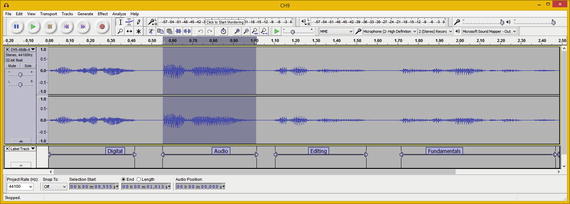
Figure 9-11.
Select vocal for the word audio, above Label Track
In Figure 9-12, you see that I selected a Size of 256 and 512 for the notch filtered (the latest version of the voice-over) data sample to show the frequency sampling resolution difference. The higher sample size shows the notch that you carved with increasing precision.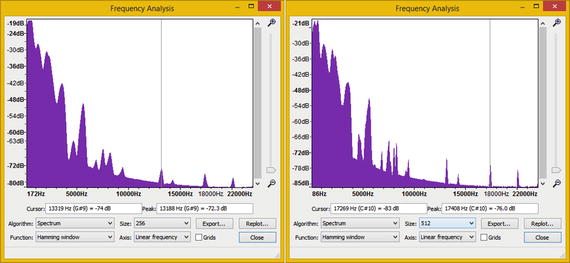
Figure 9-12.
Notch Filter spectral analysis at Size 256 and 512
It is important to note that the vertical line in your graph should “snap” to the nearest peak as you move your mouse over the data. The Cursor and Peak readouts provide precise numerical information to use with the Effect menu filters and in their audio effect dialog settings.
Next, let’s drill down yet again and use this tool on a data sub-subsample; that is, on just a small portion of a data sample, such as the first part of the word “audio” that you did surgery on in Chapter 7.
Partial Subsample Analysis: Smaller Selections
Select the first portion of the vocal “audio” word sample (see Figure 9-13), and again, invoke Analyze ➤ Plot Spectrum to analyze this snippet
(or sub-subsample).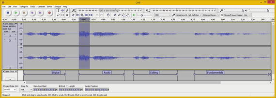
Figure 9-13.
Select an even smaller snippet on front of “audio”
As shown in the left-hand screenshot in Figure 9-14, you can see the frequency data even more clearly. The fewer data samples that you select, the more clearly you can see the frequency distribution. This is because the data has more room to spread out inside the Frequency Analysis window, as is evident on both sides of Figure 9-14. Notice that in the right-hand screenshot, I changed the Algorithm from Spectrum to Standard Autocorrelation.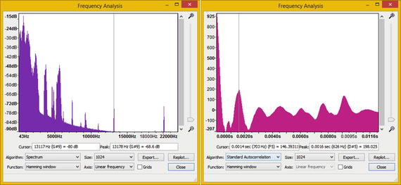
Figure 9-14.
Spectral analysis of first portion of word “audio”
In case you are wondering what these three different algorithm types do, the Spectrum algorithm, which is a default setting, plots the FFT of your audio spectrum data. FFT stands for Fast Fourier Transform; it is the algorithm that computes the Discrete Fourier Transform (DFT) of any data sequence.
Fast Fourier analysis
converts the signal (audio sample data) from its original mathematical domain, usually over time, to a spatial representation; in this case of digital audio waveforms, it is both. This allows you to visualize your data in a different way, which can be quite helpful in assisting you in your workflow decision-making process.
The three
Autocorrelation algorithm
options measure the extent to which your audio sample data repeats itself. This algorithm does this by taking two copies of the sample data and then moving one forward by one sample. These two copies are then multiplied together and all the values are summed. This is repeated for two samples difference, and so on, up to a number of samples that you specify using the size option.
Autocorrelation gives a small result if the waveform is random (such as white, pink, or Brownian noise), and a large result if it is repetitive (like a decaying, held, musical note).
By looking at peaks for this algorithm’s data plot, your key frequencies can still be determined, even if there’s a lot of noise in the data sample. Figure 9-15 shows the Standard Autocorrelation algorithm using 2048 and 4096 data sample sizes. Note that the cursor snaps to each peak frequency.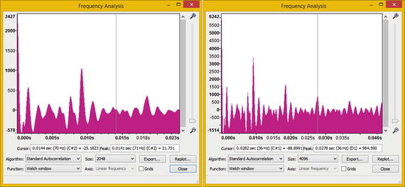
Figure 9-15.
A Welch function at 2048 or 4096 can simulate waves
The Cepstrum algorithm
for an audio signal is related to the Spectrum algorithm, but represents a rate of change across the different spectrum bands.
This algorithm is useful for ascertaining spectral properties in vocal tracks and can be used to identify speakers by their different vocal frequency characteristics!
Figure 9-16 shows the Cepstrum algorithm at a 256 samples size, using the Welch function data display. Notice that I have resized the window in the X (width) dimension to space out these data curves so that their peaks are more visually ascertainable. You should leverage this feature because you can also resize this window in the Y (height) dimension if you need to fit a different spectral data graphing view. All in all, the Frequency Analysis dialog is a very powerful data visualization tool.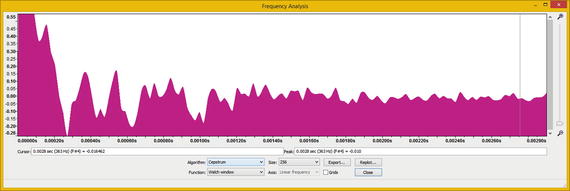
Figure 9-16.
A Cepstrum algorithm, at 256 frequency sample size
Be sure to experiment with all the different settings and features that this Plot Spectrum tool can provide for your digital audio editing.
Summary
In this chapter, you explored the Analyze menu and various algorithmic analysis tools, including the visual analysis of frequency spectrums using the Plot Spectrum tool, and tools that create Label Track data and export sample analysis data in numeric format. You looked at how to analyze progressively smaller data samples to drill down into visual analytical data representations. And you looked at the three different algorithm categories that you can use to analyze your data.
In the next chapter, you learn all about digital audio data compositing concepts and principles via Audacity’s Tracks menu.