Adaptive query processing
Approximate query processing
Table variable deferred compilation
Scalar UDF inlining
I’ve already covered other aspects of some of the Intelligent Query Processing including optimized plan forcing and Parameter Sensitive Plan Optimization in other chapters. I also covered adaptive joins in the chapter on columnstore indexes.
As wonderful as this new technology is, it won’t fix bad code choices or poor structures. Even with all these new, better, methodologies for query execution, standard tuning will still have to take place. However, even a well-tuned system will see benefits from various aspects of Intelligent Query Processing.
Adaptive Query Processing
Adaptive joins (which were already covered)
Interleaved execution
Query processing feedback
Optimized plan forcing (covered in Chapter 6)
Interleaved Execution
I have a standing recommendation to avoid using multi-statement table-valued functions and nothing I’m about to tell you about changes that recommendation. However, there is still going to be situations where you have these functions in place and your performance could suffer.
Starting in SQL Server 2017, however, Microsoft has changed the way that multi-statement functions behave. The optimizer can identify that this type of function is being executed. SQL Server can allow those functions to execute and then, based on the rows being processed, can adjust the row counts on the fly in order to get a better execution plan.
Multi-statement user-defined table-valued functions
This example is a very common antipattern (code smell) that can be found all over. It’s basically an attempt to make SQL Server into more of an object-oriented programming environment. Define one function to retrieve a set of data, a second to retrieve another, then a third that calls the other functions as if they were tables.
In older versions of SQL Server, prior to 2014, the optimizer assumed these tables returned a single row, regardless of how much data is actually returned. The newer cardinality estimation engine, introduced in SQL Server 2014, assumes 100 rows, if the compatibility level is set to 140 or greater.
Executing the functions both ways
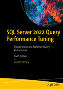
A window of the two different strategies for carrying out both query 1, query cost, relative to the branch at 1, and query 2, query cost, relative to the branch at 99 percent.
Execution plan for a non-interleaved execution and an interleaved execution
The overall shape of the execution plans is the same. However, there are very distinct differences. For example, since these queries were run as part of a single batch, each plan is measured against the other. The top plan is estimated at only 1% of the cost of the execution, while the second plan is 99%. Why is that?

A table has two columns and fifteen rows. The headers are actual execution mode and row, and 15 row entries.
Properties from the non-interleaved plan
At the top, you can see the actual number of rows as 148. At the bottom, you can see that the estimates were for 100 rows total and 3.16228 for all executions. It’s that disparity in the estimated number of rows, 3.16228 vs. 148, that frequently causes performance headaches when using table-valued functions.

A table about misc has two columns and fifteen rows for execution properties. The headers are actual execution mode and row, and 15 row entries.
Properties from an interleaved execution
Of course, the same number of rows was returned. The interesting parts are at the bottom. Instead of 100 rows, it’s clear that we’re dealing with larger data sets at 121,317. Also, instead of 3.16228, we’re seeing 18.663. While this isn’t perfect as an estimate, it’s much better, and that’s the point.
The differences in execution times between these are trivial. The non-interleaved execution was approximately 785ms with 371,338 reads. The interleaved execution was 725ms with 349,584 reads. The improvement was small, but it is there.
An improved multi-statement function
Using parameters instead of a WHERE clause
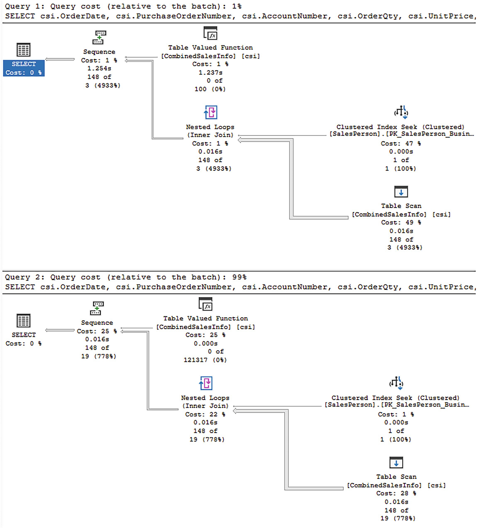
A diagram begins from the right with clustered index seek at 8%, 0.000 seconds, 17 of 17 at 100, and table scan at 13, 0.000 seconds, 148 of 148 at 100, and table valued function at 1, 0.000 seconds, 0 of 148 at 0 to sequence cost at 1, 0.000 seconds, 148 of 148 at 100 percent, ends with the selection at 0 percent cost.
A new execution plan with better estimates
The estimated number of rows and the actual number of rows perfectly match. Further, the plan has changed from using a Loops Join to a Hash Match since that will be more effective for the amount of data involved.
Performance went down to 7.8ms with 1,120 reads, an enormous improvement. However, it’s worth noting that the non-interleaved performance improved as well. It was 8.1ms with 1,414 reads. So we’re still only talking about .3ms improvement here. As before, faster is faster, and no code changes are required to get the improved performance since interleaved execution is just a part of the engine now.
One more thing to keep in mind when talking about interleaved execution, especially using parameters like this. The plan created is based on the parameters supplied and the data they’ll return. That plan is stored in cache. To a degree, this can act like parameter sniffing if you have a wildly varying data set. This is why you have the ability to turn off interleaved execution if you need to. You can also turn it off through a query hint.
Query Processing Feedback
Memory grants
Cardinality estimates
Degree of parallelism
Feedback persistence
Memory Grants
When introduced, memory grant feedback worked only for batch mode processing. In SQL Server 2019, row mode memory grant feedback was also introduced. Part of the calculations from the optimizer is the amount of memory that will need to be allocated to execute a query. If not enough memory gets allocated, then the excess data gets written out to disk through tempdb in a process called a spill. If too much memory is allocated, the query is simply using more than it should. Either way, both these scenarios lead to performance issues.
SQL Server can now adjust the memory allocation after analyzing how memory was used during the execution of the query. Adjustments can be made, up or down, to ensure better performance and better memory management.
Creating an Extended Events session for memory grant feedback
For this session, in the event a query is suffering from parameter sensitivity, also known as parameter sniffing, memory grant feedback could be all over the map. The engine can recognize this, and the memory_grant_feedback_loop_disabled event will fire for that query. When a query experiences changes in its memory allocation due to feedback, the next event, memory_grant_updated_by_feedback, will return information about the feedback process. Finally, I have the sql_batch_completed event so I can see the query associated with the other events, and I have it all tied together through Causality Tracking (explained in Chapter 3).
Creating the CostCheck procedure

Table 1 has four columns and two rows; the highlighted entries are under the first row. Table 2 has two columns and 13 rows, the headers are field and value, and 13 row entries.
Results of memory grant feedback
A few points are illustrated here. First, by looking at the sequence from Causality Tracking, we can tell that the memory grant feedback occurs before the query finishes executing. We can see, right at the bottom, the amount of memory granted was 75,712, but the memory used was 11,392, a large overallocation. Anything where the allocated memory is more than twice the used memory is considered an overallocation.
However, if you execute the procedure a second time with the same value, you’ll find that no memory_grant_updated_by_feedback event occurs. This is because the memory grant has been adjusted and is now stored in cache with the plan.
If you execute the procedure with a different value, say 117.702, which returns only one row (as opposed to over 9,000), the memory grant is not readjusted. This is because the difference is small enough it doesn’t require a readjustment.
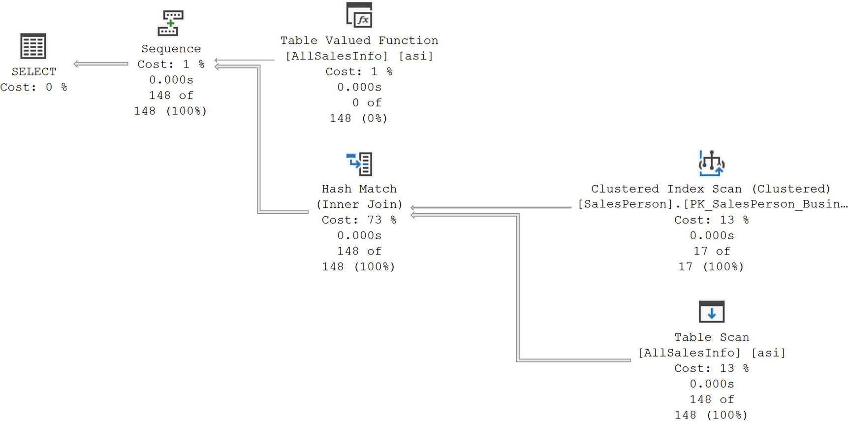
A table of memory grant info has 2 columns and 11 row entries. Highlighted is row entry 4 which reads is memory grant feedback adjusted, yes stable.
Evidence of memory grant feedback within an execution plan
YesAdjusting: Memory grant feedback has been applied, and it may change in future executions.
NoFirstExecution: Memory grant feedback is not generally applied during the first compile and execution.
NoAccurateGrant: There has been no spill, and more than half the allocated memory is in use.
NoFeedbackDisabled: There has been thrash; memory adjusts up and down multiple times, probably from parameter sniffing or statistics issues; and memory feedback is disabled.
Disabling memory grant feedback
Memory grant feedback is completely cache dependent. If a plan with feedback is removed from cache, when it is recompiled, it will have to go through the feedback process again. However, it is possible to store this information in Query Store. I’ll discuss that in a separate section on feedback persistence later in the chapter.
This example was a batch mode execution, but the row mode processing is exactly the same in both behavior and how to monitor it using extended events.
Finally, prior to SQL Server 2022, memory grant feedback was subject to some thrash, meaning if a query needed more memory, it was granted. Then, if the next execution required less, it was cut back again. This can lead to poor performance. So in SQL Server 2022, the memory grant is adjusted as a percentile over time, not as a raw number. That then arrives at a better place for performance. This behavior is on by default, and there’s nothing you have to do to enable it. If you choose to disable it, you can alter the database scoped configuration using the MEMORY_GRANT_FEEDBACK_PERCENTILE = OFF command.
Cardinality Estimates
Starting with SQL Server 2022, the cardinality estimates can benefit from a feedback process. The compatibility mode for the database has to be 160 or greater, and Query Store must be enabled. The reason for this is the feedback mechanism uses Query Store hints (described in Chapter 6) to adjust how cardinality is estimated.
Observing CE feedback
There are a limited number of scenarios that are likely to lead to a situation where (CE) feedback can help. The first of these is in dealing with data correlation. In the old cardinality estimation engine (compatibility 70), prior to SQL Server 2014, the assumption was that there is no correlation between columns within a table. The modern cardinality estimation engine (compatibility 120 or greater) assumes a partial correlation between columns. There are of course situations where there is direct correlation between the data in columns as well. CE feedback will look at if the data is underestimated or overestimated compared to the actual rows. It will then apply hints through the Query Store to get better row estimates for the plan.
Filtering on two columns in the table

A table has two columns and four rows. The headers are name and timestamp, and four row entries.
CE feedback events caused by a query

A table of details about the event query telemetry has two columns and 17 rows. The headers are field and value and 17 row entries.
query_ce_feedback_telemetry
This shows you the data that is being used as a part of the CE feedback process. The columns cover all three scenarios, not just the first one. I’ve included this for informational purposes. There’s not a lot here that you can use for evaluating your own queries or system behaviors. However, you can use it to have the data that Microsoft is using internally.
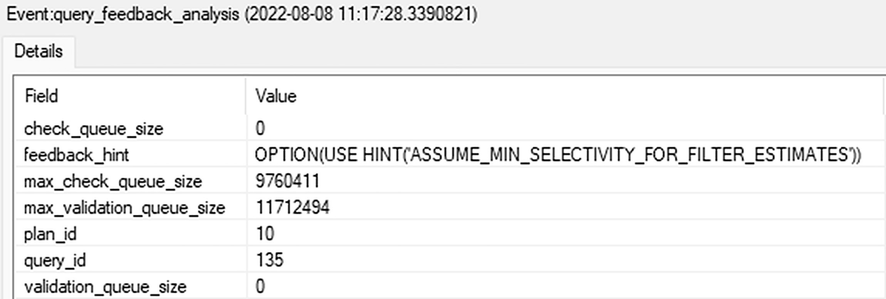
A table of details about the event query feedback analysis has two columns and seven rows. The headers are field and value and seven row entries.
query_feedback_analysis
Here, you get the hint that will be used to address the functionality. You also get the plan_id and query_id so you can pull the information straight from the Query Store.
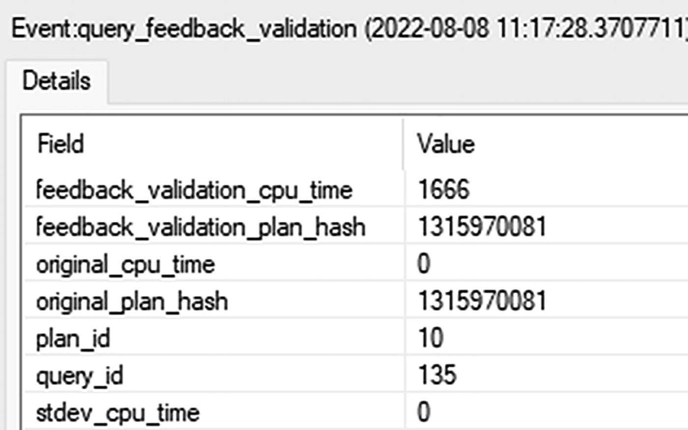
A table of details about the event query feedback validation has two columns and seven rows. The headers are field and value and seven row entries.
query_feedback_validation
The important information here is the two hash values. In this case, they’re the same, showing that while this query was evaluated for CE feedback, no hint was applied at this time.
Retrieving data from sys.query_store_plan_feedback

A table has six headers and one row. The headers are query s q l text, feature i d, feature description, feedback data, state, and state description, and row 1 first entry is highlighted.
Status of CE feedback on a query
The most important information here is the state_desc that lets us know that after evaluation, the plan was regressed back to its original.
The next condition applies to row goals. When a query specifies that a specific number of rows are going to be returned, such as when using the TOP operator, then the optimizer will limit all estimates to be below the goal count. However, in the case where data is not uniformly distributed, the row goal may become inefficient. In that case, the CE feedback can disable the row goal scan.
Querying the bigProduct table with a TOP operation
Executing this 17 times does get me a query_ce_feedback_telemetry event. I also get an entry in sys.query_store_plan_feedback. However, the result is NO_RECOMMENDATION. The evaluator for the CE decided that even attempting a hint wouldn’t be worth it on this query.
The final scenario is related to join predicates. Depending on the CE engine, either 70 or 120 and greater, different assumptions are made regarding the correlation of join predicates. The old behavior was similar to compound keys, full correlation is assumed, and the filter selectivity is calculated and then the join selectivity. This is referred to as Simple containment. The modern CE assumes no correlation, base containment, where the join selectivity is calculated first and then the WHERE and HAVING clauses get added.
Querying the bigProduct and bigTransactionHistory tables
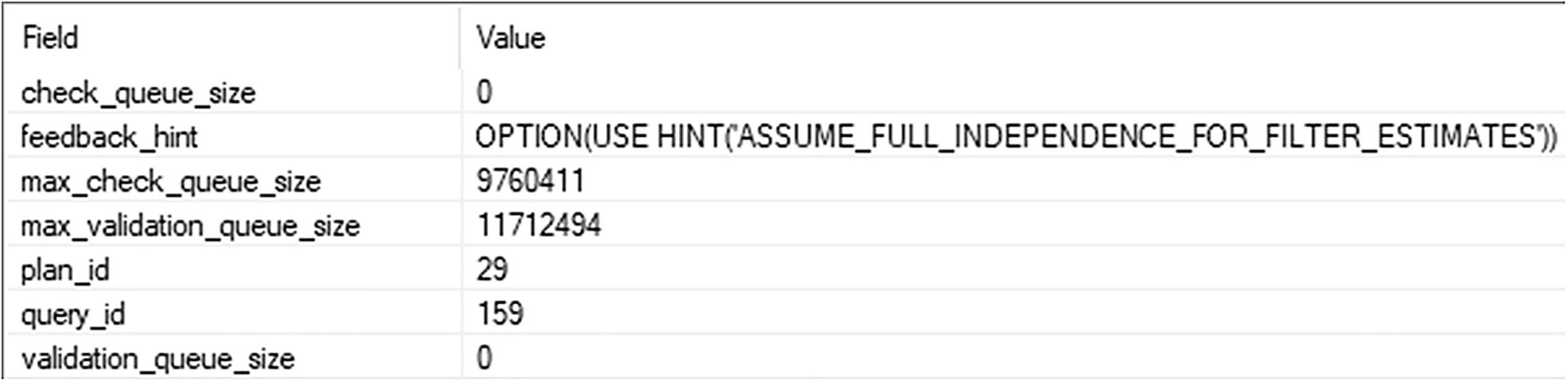
A table has two columns and seven rows. The headers are field and value, and seven row entries.
New feedback hint being evaluated
So there is the new hint, ASSUME_FULL_INDEPENDENCE_FOR_FILTER_ESTIMATES; in short, it tested whether simple containment would work better for this query.
You can disable CE feedback using ALTER DATABASE SCOPED CONFIGURATION SET CE_FEEDBACK = OFF. You can turn it back on the same way. You can also pass a query hint, DISABLE_CE_FEEDBACK.
If you have a hint in the query, you’re using Query Store hints, or you’re forcing a plan, CE feedback won’t occur. You can, however, override the hints using database scoped configuration again, this time setting FORCE_CE_FEEDBACK = ON.
Degree of Parallelism (DOP) Feedback
Parallel execution of queries can be extremely beneficial for some queries. However, there are other queries that suffer badly when they go parallel. As I discussed in Chapter 2, the best way to deal with getting the right plans to go, or not go, parallel is to use the Cost Threshold for Parallelism. Even then, some queries that exceed that threshold may still suffer from poor performance due to parallelism.
Turning on DOP feedback
Extended Events session for monitoring DOP feedback
Setting up a demo for DOP Feedback is complicated. It requires even more data than we’ve loaded into AdventureWorks so far. Instead of listing all the required code here, making the book artificially larger, I’m going to suggest you reference this example by Bob Ward: bobsql/demos/sqlserver2022/IQP/dopfeedback at master · microsoft/bobsql (github.com).
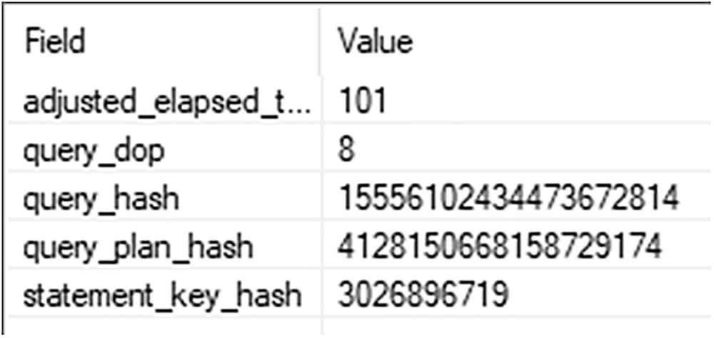
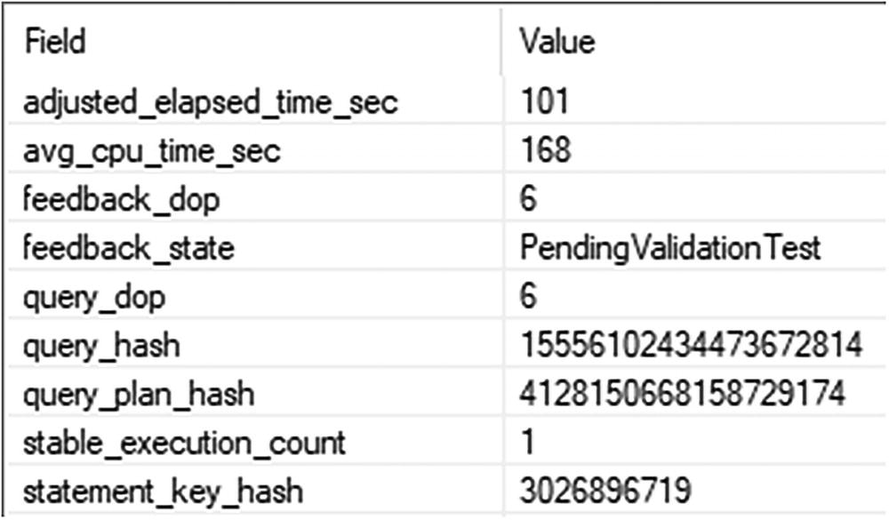
A table has two columns and five rows. The headers are field and value, and five row entries.
A query that may benefit from DOP feedback

A table of the change in the query's D O P has two columns and nine rows. The headers are field and value, and nine row entries.
A suggested change to the DOP for this query
There is useful information here to help you track which query, which statement, the plan, etc. However, the interesting piece is the fact that the query DOP has been 8 and is now suggested to be better at 6.
A table of the validation of the D O P change has two columns and nine rows. The headers are field and value, and nine row entries.
Validating that the suggested DOP change is working
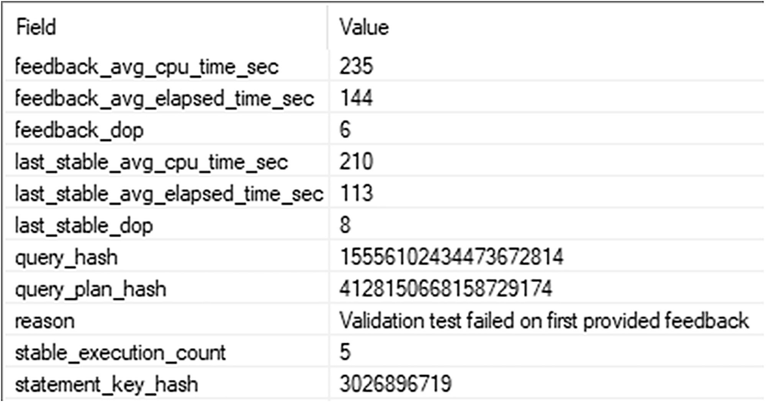
A table of the D O P reverts after a failed validation has two columns and 11 rows. The headers are field and value, and 11 row entries.
A failed validation where the DOP reverts back
After five executions, performance didn’t improve, so the optimizer has reverted back to the last stable DOP, a value of 8. You can see that the query is running on average; slower during the test. The feedback_avg_cp_time_sec is at 235 and slower than last_stable_avg_cpu_time_sec of 210. The average elapsed time is also slower.
The engine will try this more than once. After it achieves an actual improvement, it will lock it in to place. The lowest it will go is a DOP value of 2.
Feedback Persistence
The ability to get feedback on memory, statistics, and degree of parallelism and then adjust query behavior based on the feedback is actually pretty wonderful. However, prior to SQL Server 2022, that feedback did not persist, meaning when a query went out of cache, any history of it having benefited from feedback was lost. Now, with Query Store, by default, the feedback is persisted to the Query Store. This means when a query is removed from cache, for whatever reason, when it gets recompiled, the existing feedback applied to the query is used again when compiling the new plan. This is a massive win in regard to performance with all the feedback processes.
Only feedback that has been validated is written out permanently. Otherwise, it’s in evaluation and won’t be persisted until it passes.
You can disable this behavior using database scoped configuration settings through MEMORY_GRANT_FEEDBACK_PERSISTENCE = OFF. When you set this to OFF, it’s off for all the feedback mechanisms. They’re all driven through this one setting.
Approximate Query Processing
APPROX_COUNT_DISTINCT
APPROX_PERCENTILE_CONT
APPROX_PERCENTILE_DISC
Unlike a lot of the other aspects of Intelligent Query Processing, the approximate functions require a change to code.
APPROX_COUNT_DISTINCT
Comparing COUNT and APPROX_COUNT_DISTINCT
The performance here is slightly better for the APPROX_COUNT_DISTINCT. The goal for this function is to deal with large data sets, in the millions of rows, and to avoid spills that are common with a COUNT(DISTINCT…) query.
Documentation says that a 2% error rate is likely with a 97% probability. In short, it’s going to be close in places where close works well enough.
APPROX_PERCENTILE_CONT and APPROX_PERCENTILE_DISC
Comparing the functions and the approximate functions
The most important aspect of the APPROX* functions is that you are not guaranteed the same result set from one execution to another. They both use a random sampling process that means they won’t be working from the same data set every time.
Execution times here are pretty severe. The first query runs about 43 seconds. The second runs in 3.2. Reads for the first query are 303,481. The second query has a varying number of reads as it randomly samples the data. However, generally, it was half, about 150,000 reads.

Two tables have three columns and five rows each. The headers are name, median cont., median disc, and five row entries.
Accuracy from the approximate functions
This is consistent with Microsoft’s claim that this function will be 1.33% accurate. At least based on the values in the figure, it’s doing well.
Table Variable Deferred Compilation
The strength of table variables is the fact that they do not have statistics. This makes them a great choice in scenarios where statistics are not needed and would be painful due to maintenance overhead and recompiles. However, the one weakness of table variables is that they don’t have statistics, so the optimizer just makes assumptions about how many rows will be returned: one (1) row. With deferred compilation, the plan involving a table variable isn’t completed until actual row counts are available to provide better choices to the optimizer, similar to how temporary tables work, but without the added overhead of recompiles.
To be able to take advantage of deferred compilation, the compatibility level has to be 150 or greater. Also, you can use database scoped configuration to disable deferred recompile, DEFERRED_COMPILATION_TV = OFF. That must be enabled.
Executing without and with deferred compilation
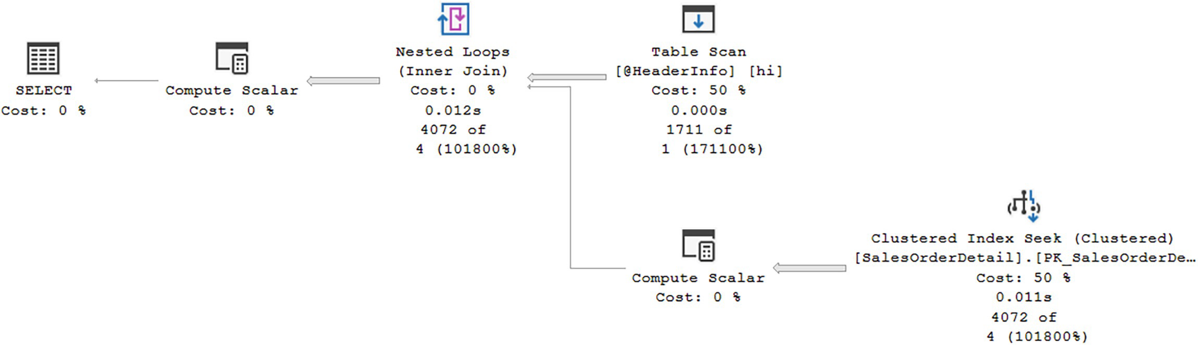
A diagram begins from the right with clustered index seek at 50 percent, 0.011 seconds, 4072 of 4 at 101800 to compute scalar at 0% and table scan at 50, 0.000 seconds, 1711 of 1 at 171100 to inner join nested loops at 0, 0.012 seconds, 4072 of 4 at 101800% to compute scalar at 0%, ends with the selection at 0 percent cost.
Row counts reflecting the estimate of one row
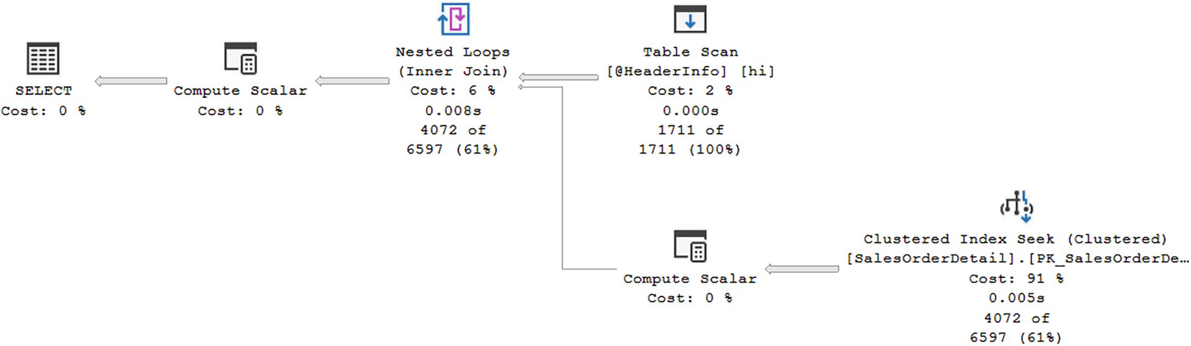
A diagram begins from the right with clustered index seek at 91, 0.005 seconds, 4072 of 6597 at 61 to compute scalar at 0 and table scan at 2, 0.000 seconds, 1711 of 1711 at 100 to inner join nested loops at 6, 0.008 seconds, 4072 of 6597 at 61 to compute scalar at 0, ends with the selection at 0 percent cost.
Deferred compilation results in more accurate row counts
While the plan shape in this example didn’t change, you can see that the plan is now based on accurate row counts. The Table Scan now shows an estimated value of 1,711 as well as the actual identical count.
Deferred compilation doesn’t increase recompile frequency. You may not always see improvements in performance. In fact, if you have a wildly varying row count for your table variables, you may see no benefit from deferred compilation at all.
Scalar User-Defined Function Inlining
User-defined functions can often be a source of problems. I talked earlier about multi-statement, table-valued functions, user-defined functions (UDF), and their inherent problems (partially addressed through interleaved execution). While inline table-valued functions can perform just fine, they can also be abused. Scalar UDFs are also something that can be a fine tool or can be abused.
The issue with scalar functions is that by their nature, they have to be applied to each row in the query. Some scalar functions, such as simple arithmetic, formatting, and something similar, will perform perfectly fine. Other scalar UDFs, such as ones that independently access data, can perform quite poorly.
The poor performance comes from multiple sources. As already mentioned, each row will get an execution of the function in an iterative fashion. Since scalar functions aren’t relational, they are not properly costed by the optimizer, which can lead to poor choices. Also, each UDF statement is compiled independently of the rest of the query, potentially missing out on optimizations. Finally, UDFs under the old system are executed serially, with no parallelism, further degrading performance potential.
Starting in SQL Server 2019 (which means a compatibility level of 150 or greater), scalar UDFs are automatically transformed into scalar subqueries. Because they are subqueries, they can be optimized with the rest of the query. This means most of the standard issues with scalar functions are eliminated.
Not all scalar functions can be transformed to inline. In fact, there is a lengthy set of exceptions outlined in the Microsoft documentation here: https://docs.microsoft.com/en-us/sql/relational-databases/user-defined-functions/scalar-udf-inlining?view=sql-server-ver16.
Scalary UDF dbo.ufnGetProductStandardCost
Validating whether a query can be executed inline
When a value of 1 is returned from sys.sql_modules, it means the scalar function can be executed inline.
Executing the scalar UDF within a query

A window depicts the two different strategies for carrying out both query 1, query cost, relative to the branch at 14, and query 2, query cost, relative to the branch at 86 percent.
Inline scalar function vs. not inline
Don’t worry about trying to read the details of the plan. There are a few simple facts that are immediately apparent. First, the plan for the UDF executed without being inline has a missing index suggestion, which is absent from the other plan. This implies that the second plan’s optimization is probably better since all the indexes it needed were available to it.
Next, you can see that the second execution went parallel. This probably also helped to enhance performance.
Finally, and you’d have to break down the plan into detail to see it, the location of the production of the data from the UDF queries has moved. In the original plan, the queries necessary to satisfy the UDF are done at the very end of execution, whereas they’re done sooner throughout the second plan. Also, there is no Compute Scalar operator for the UDF in the second plan.
Obviously, since the plan has changed, things like hints, the query and plan hash, and dynamic data masking may all work differently. You may also see warnings that were previously masked inside the plan for the scalar function (by the way, that plan can be seen by looking at the Estimated Plan for a query using a scalar function).
While some queries may not benefit from this functionality, clearly, others will.
Summary
Intelligent Query Processing covers a lot of ground, from automated feedback, to changes in the query itself, to code changes that can better support performance. Don’t forget that as excellent as this functionality is, and it is excellent, it won’t fix bad code or incorrect structures. Standard query tuning is still going to be a part of the process. However, where you have common issues, there may be some solutions that simply occur automatically, thanks to Intelligent Query Processing.
Speaking of automated fixes, the next chapter will cover automated tuning in SQL Server and Azure SQL Database.