In-Memory OLTP Fundamentals

Disks, disk controllers, and the whole architecture around permanent storage of the information that SQL Server manages have gone through radical changes over the last few years. As such, storage systems are blazingly fast. And yet, it is still possible to have systems that bottleneck on the storage systems.

At the same time, memory operations have also improved equally radically. The amount of memory that can be put on systems has increased in enormous ways, making memory even faster than disks. However, never forget, memory is only, ever, temporary storage. If you want your data persisted, it has to have a way to get to the disk.

Microsoft recognized that in order to make transactions faster, they would have to remove the pessimistic locks on data. The in-memory tables use an optimistic locking approach. They’re using a data versioning scheme to allow multiple transactions to write data, with a “last one in wins” kind of approach. That eliminates all sorts of locking and blocking.

Additionally, instead of forcing all transactions to wait until they are written to the log to complete, an assumption is made that most transactions complete. Therefore, log writes occur asynchronously so that they don’t slow down transactions for the in-memory tables.

Yet another step was to make memory management itself optimistic. In-memory tables work off an eventually consistent model. There is a conflict resolution process that could roll back a transaction but won’t allow a transaction to block another. All operations within memory-optimized tables are then subsequently faster.

Additionally, internally, they’ve changed the way that the buffer pool works so that there are optimized scans for systems with extremely large memory pools. Without this, you would simply be moving where the slowdown occurs.

Finally, in addition to all the optimizations to data access, Microsoft added natively compiled stored procedures. This is T-SQL code that is turned into a DLL and run within the SQL Server OS. There is a lengthy, and expensive, compile process, but then, execution is radically enhanced, especially when working with the memory-optimized tables.

Best of all, largely, you can treat memory-optimized tables largely the same way you treat other tables, although you can’t do just anything you want. There are a number of limitations on behaviors and some specific system requirements.

Creating Tables

The primary magic is in the WITH statement. First, I’m identifying this table as being specifically MEMORY_OPTIMIZED. That will ensure that it goes to the correct file group. Additionally, I’m defining my durability, here a fully durable table supporting both schema and data.

The next thing worth noting is the index. This is not one of the indexes we’ve referenced throughout the book. This index, NOCLUSTERED HASH, is unique to memory-optimized tables. We’ll drill down on indexing a little later in the chapter.

Otherwise, all the data types are supported. You can also use foreign keys, check constraints, and unique constraints ever since SQL Server 2016. Also, memory-optimized tables support off-row columns, meaning a single row can be greater than 8060 bytes.

Another limitation is that a memory-optimized table can’t take part in a cross-database query. Therefore, in order to load the data, I created a staging table. There may be ways to optimize this process, but it should be noted the cross-database query took 77ms and the query to load the in-memory table only took 18ms, for the same data.

Notice, this is a mix of memory-optimized tables and a standard SQL Server table. Yet the query runs just fine. We can even capture an execution plan with runtime metrics in Figure 19-1.

A diagram begins on the right with 2 non-clustered hash index seek with values of, 1% cost, 0.000 seconds, and 1 of 1, each, and a clustered index seek with values 99% cost, 0.000 seconds, and 1 of 1, given.

The best part is that the optimizer thinks that the single row, Clustered Index Seek, against the standard clustered index is 99% of the cost of the query.

However, the important point here is how mundane this is. It’s just an execution plan. Yes, it has seeks against a nonclustered hash table instead of any of the indexes we’ve covered throughout the book, but if you’ve read straight through to this point, you know what an index seek represents. It’s no different because it’s in memory-optimized tables.

This is a very small example returning a single row, but approximately 22% faster, and a 66% reduction in reads indicates the possibility of other performance enhancements as other queries get run.

One point I need to make here. The reads that we’ve been using throughout the book are not the same as reads with memory-optimized tables. No data is read off of disk except during the recovery of the database during startup or failover. That means while we still have the value of reads, we can’t do what I just did, a straight comparison on those reads. Fewer reads with memory-optimized tables are better, of course, but it’s not the same values. Duration is your better comparison measurement, at least when comparing traditional behaviors with the in-memory ones.

In-Memory Indexes

Every memory-optimized table must have one index. Since the row is stored as a unit within the in-memory table, an index has to be there in order to make a table. The data is not stored on a page, which is why reads are not the same. Because of this, there is no worry about index fragmentation. An UPDATE consists of a logical DELETE and an INSERT. A process comes along later to clean things up.

Prior to SQL Server 2017, you were limited to eight indexes per table. Now, the limit is 999 (but remember, it’s a limit, not a goal).

The indexes on a memory-optimized table live in memory in the same way that the table does. Their durability matches that of the table they’re created on.

Let’s explore these indexes in more detail.

Hash Index

The hash index is different from the other index types within SQL Server. A hash index uses a calculation to create a hash value of the key. The hash values are stored in buckets, or a table of values. The hash calculation is a constant, so for any given value, the same hash value will always be calculated.

Hash tables are very efficient. A hash value is a good way to retrieve a single row. However, when you start to have a lot of rows with the same hash value, that efficiency begins to drop.

The key to making the hash index efficient is getting the correct distribution across your hash buckets. When you create the index, you supply a bucket count. In the example in Listing 19-3, I supplied a value of 50,000 for the bucket count. When you consider there are currently about 19,000 rows in the table, I’ve made the bucket count more than big enough to hold the existing data, and I left room for growth over time.

The bucket count has to be big enough without being too big. If the bucket count is small, a lot of values are inside a single bucket, making the index less efficient. If you have a lot of empty buckets, when a scan occurs, they are all read, even though they are empty, slowing down the scan.

Figure 19-2 illustrates how hash buckets work.

A diagram on top labeled large bucket count has a row of 6 buckets, where buckets 1, and 3 to 6 contain bricks labeled hash values 1 to 5, and bucket 2 is empty. The diagram below labeled, small bucket count, has a row of 6 buckets.

The first set of buckets is what is defined as a shallow distribution. That is to say, a few hash values distributed across a lot of buckets. The second set of buckets at the bottom of Figure 19-2 represents a deep distribution. In that case, fewer buckets with more values in them.

With a shallow distribution, point lookups, individual rows, are going to be extremely efficient, but scans will suffer. Whereas in the deep distribution, point lookups won’t be as fast, but scans will be faster. However, if you are in a situation where your queries are doing a lot of scans of a memory-optimized table, you may want to switch back to a regular table again.

The recommendation for bucket counts completely depends on your data and your data growth. If you don’t expect any data growth at all, set the number of buckets equal to your row count. If your data is going to grow over time, set it somewhere between one and two times the row count. Don’t worry too much about this. Even with too many, or too few, buckets, performance is likely to be great. Just remember, the more buckets you allocate, the more memory you’re using.

You also have to be concerned with how many values can be returned by the hash value. Unique indexes and primary keys are excellent choices for a hash index because their values will be unique. The general recommendation is a ratio of total rows to unique values being less than 10.

The hash value is simply a pointer to the bucket. If there are multiple rows, they are chained together, each row pointing to the next row. When a bucket is found, you’ve found the first value in the chain. You then scan through the chain to find the actual row you’re interested in. This means a point lookup turns into a bit of a scan, hence keeping the number of duplicates in the hash to a minimum.

You can see the distribution of your data within the hash index using the query in Listing 19-7.

SELECT i.NAME AS [index name],

       hs.total_bucket_count,

       hs.empty_bucket_count,

       hs.avg_chain_length,

       hs.max_chain_length

FROM sys.dm_db_xtp_hash_index_stats AS hs

    JOIN sys.indexes AS i

        ON hs.OBJECT_ID = i.OBJECT_ID

           AND hs.index_id = i.index_id

WHERE OBJECT_NAME(hs.OBJECT_ID) = 'Address';

Listing 19-7

Querying sys.dm_db_xtp_hash_index_stats

The results are in Figure 19-3.

A table has 5 columns and 1 row with headers, index name, total bucket count, empty bucket count, average chain length, and max chain length. The row entries are P K underscore address underscore 091 C 2 A 1 A 604 E D F A 2, 65536, 48652, 1, and 5.

There are several imports pieces of information here. First you should note the total_bucket_count value of 65,536. I called for 50,000 buckets, but SQL Server rounded it up to the next power of 2 value. I have about 48,652 empty buckets, which is a little high, but maybe I’m anticipating growth. The average chain length is 1, which is very good. The maximum chain length is 5, which is good enough being below 10.

If there were even more empty buckets, the average chain length was above 5 and max chain length was greater than 10, it might be time to consider a nonclustered index for the memory-optimized table.

Nonclustered Indexes

A nonclustered index on a memory-optimized table is no different than a nonclustered index on a regular table, other than where the data is stored. Durability again will be dictated by the durability of the table.

Consider the query in Listing 19-8.

SELECT A.AddressLine1,

       A.City,

       A.PostalCode,

       sp.NAME AS StateProvinceName,

       cr.NAME AS CountryName

FROM dbo.ADDRESS AS A

    JOIN dbo.StateProvince AS sp

        ON sp.StateProvinceID = A.StateProvinceID

    JOIN dbo.CountryRegion AS cr

        ON cr.CountryRegionCode = sp.CountryRegionCode

WHERE A.City = 'Walla Walla';

Listing 19-8

A query in need of an index

Running this query results in the execution plan in Figure 19-4.

A diagram on top begins with a table scan with values 73% cost, 0.005 seconds, and 19614 of 19614 given, to filter at 8% cost, 2 nested loops at 0% cost each, and select at 0%.

Because the WHERE clause is unsupported by any index, we’re getting a scan of the dbo.Address table. While a scan of an in-memory table will be faster than one stored on disk, it’s still a performance issue in the same way it would be on another query.

You can’t simply run CREATE INDEX on a memory-optimized table. Instead, you have to either recreate the table or use ALTER TABLE as a way to add an index. Listing 19-9 shows how.

ALTER TABLE dbo.ADDRESS ADD INDEX nci (City);

Listing 19-9

ALTER a memory-optimized table to add an index

Running the query from Listing 19-8 again results in a different execution plan (Figure 19-5).

A diagram on top begins with 2 non-clustered index seek with values of 9% cost, 0.000 seconds, 100 of 100, and 7%, 0.000 seconds, 100 to 100, given, respectively, to 2 nested loops at 2% cost each, and select at 0%.

The nonclustered index replaces the scan. Because of how the data is stored in a memory-optimized table, no Key Lookup operation is needed. Performance went from 5.9ms to 1.1ms, a considerable gain.

Columnstore Index

There are no major distinctions between a memory-optimized table and a regular table when it comes to a columnstore index. You are limited to only a clustered columnstore. You have to have the memory to support the data stored in the index. Otherwise, it’s just a columnstore index.

Statistics Maintenance

Memory-optimized tables still have statistics, and those statistics must be maintained. Information about the statistics can be gathered using standard means. Listing 19-10 shows the properties of the statistics on the Address table.

SELECT s.NAME,

       s.stats_id,

       ddsp.last_updated,

       ddsp.ROWS,

       ddsp.rows_sampled,

       ddsp.unfiltered_rows,

       ddsp.persisted_sample_percent,

       ddsp.steps

FROM sys.STATS AS s

    CROSS APPLY sys.dm_db_stats_properties(s.OBJECT_ID, s.stats_id) AS ddsp

WHERE s.OBJECT_ID = OBJECT_ID('Address');

Listing 19-10

Querying sys.dm_db_stats_properties

The results from my table are in Figure 19-6.

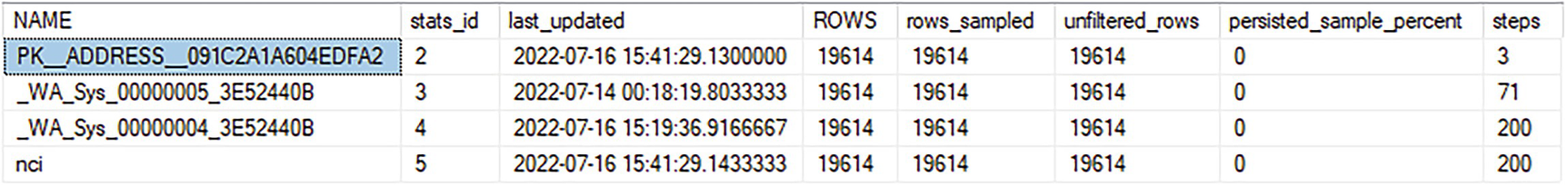
A table has 8 columns and 4 rows with headers, name, stats i d, last updated, rows, rows sampled, unfiltered rows, persisted sample percent, and steps. The first entry under the name column is P K underscore address underscore 091 C 2 A 1 A 604 E D F A 2, and is highlighted.

As you can see, statistics are created for the indexes on the table, but also system-generated statistics are created. You can use standard mechanisms to look at the data within the statistics, including hash indexes. Listing 19-11 shows a query for retrieving a histogram from the hash index.

SELECT ddsh.step_number,

       ddsh.range_high_key,

       ddsh.range_rows,

       ddsh.equal_rows,

       ddsh.distinct_range_rows,

       ddsh.average_range_rows

FROM sys.dm_db_stats_histogram(OBJECT_ID('Address'), 2) AS ddsh;

Listing 19-11

Querying sys.dm_db_stats_histogram

This returns the values shown in Figure 19-7.

A table has 6 columns and 3 rows, with column headers step number, range high key, range rows, equal rows, distinct range rows, and average range rows. The first row entries are 1, 1, 0, 1, 0, 1, where the first entry is highlighted.

Statistics are automatically maintained in SQL Server 2016 and greater as long as the database compatibility level is set to at least 130. Prior to that, or with the compatibility level set lower, you will have to maintain statistics manually.

You can use sp_updates or UPDATE STATISTICS. However, in SQL Server 2014, you will have to use FULLSCAN or RESAMPLE along with RECOMPUTE as shown in Listing 19-12.

UPDATE STATISTICS dbo.ADDRESS

WITH FULLSCAN,

     NORECOMPUTE;

Listing 19-12

Updating statistics in 2014

Otherwise, you will generate an error.

Apart from that exception, statistics are largely the same as described in Chapter 5.

Natively Compiled Stored Procedures

Executing the natively compiled procedure for the value of ‘Walla Walla’ in the same way as Listing 19-8 results in a query running in 794mcs compared to the 1.1ms from before.

There are other restrictions and requirements visible in the code in Listing 19-13. First, parameters cannot accept NULL values. You have to enforce schema binding to the underlying tables. Finally, the procedure must exist within an ATOMIC BLOCK. Atomic blocks require that all statements within the transaction succeed, or all statements within the transaction get rolled back.

Starting in SQL Server 2019, you can capture execution plans with runtime metrics, also called Actual Plans. You can also see estimated plans. Figure 19-8 shows the plan from this procedure.

The diagram on top begins with a non-clustered index seek and a non clustered hash index seek at costs of 6% and 3%, respectively, to 2 nested loops, compute scaler, and select.

The plans for natively compiled procedures are created when you create the procedure. These plans look the same, but there are some differences in the properties. Figure 19-9 shows the SELECT operator properties from the plan.

A table titled M i s c has two columns and five rows. The entries in the fifth row are in bold fonts and read as, statement, select A, dot, address line 1, comma, A, dot, city, comma.

Because this procedure executes within the OS, most of the properties we’re used to seeing aren’t applicable.

You should use execution plans the same way as you would with a regular query. You’ll see where there may be optimization opportunities looking for scans, etc. One note, all join operations within a natively compiled procedure will be Nested Loops. No other join operations are supported.

Recommendations

While the performance enhancements of memory-optimized tables and natively compiled procedures are simply huge, you should not simply, blindly, start migrating your databases and objects to in-memory. There are serious hardware requirements that you must meet. Here are a number of considerations you should work through prior to implementing this technology.

Memory Optimization Advisor

As a way to help, Microsoft has supplied functionality within SSMS that will test individual tables for supporting a move to in-memory. Right-clicking a table and selecting “Memory Optimization Advisor” from the context menu is all that is required. Figure 19-10 shows the information from the Person.Address table in the AdventureWorks database.

A window has a table with three columns and fourteen rows. The first column contains X, check, and warning symbols.

Because the Geography data type isn’t allowed in memory-optimized tables, this fails the initial test. You can see that it passed several other tests and received a warning that for a migration scenario, other tables would have to be processed without foreign keys.

In order to see the next steps, I’ll use Listing 19-15 to create a test table in the InMemory database.

USE InMemoryTest;

GO

CREATE TABLE dbo.AddressMigrate

(

    AddressID INT NOT NULL IDENTITY(1, 1) PRIMARY KEY,

    AddressLine1 NVARCHAR(60) NOT NULL,

    AddressLine2 NVARCHAR(60) NULL,

    City NVARCHAR(30) NOT NULL,

    StateProvinceID INT NOT NULL,

    PostalCode NVARCHAR(15) NOT NULL

);

Listing 19-15

Setting up a table for migration to memory optimized

The table shown in Figure 19-11 passed the initial checks.

A window has a table with three columns and nine rows. The first column has check marks as entries in all rows, and the second column contains entries like, a table is not partitioned or replicated, and no sparse columns are defined, among others.

Next, Microsoft supplies a series of warnings for the migration to memory optimized (Figure 19-12).

A window has a table with 3 columns and 5 rows. The first column has the information icon as entries in all rows, and the second column contains entries like truncate table and merge statements cannot target a memory-optimized table, among others.

It doesn’t simply perform the checks and warnings, it will actually migrate the table. Next, you get the options for naming and data migration (Figure 19-13).

A dialog box contains the following, memory-optimized filegroup, logical file name, file path, rename the original table, and estimated current memory cost in megabytes, among others. A tick mark is next to the text, also copy table data to the new memory optimized table.

After that, since every memory-optimized table must have an index, you choose which type of index you want for your table (Figure 19-14).

A dialog box contains the following, a 2 column table with headers column, and type, with the entry, address I D ticked and highlighted, and the selected option, use a non clustered hash index, among others.

You will need to supply a bucket count if you’re using the hash index. At this point, you can generate a report, or a script that does all the work, or you can click the Migrate button and see it all go. Figure 19-15 shows the results of clicking that button.

A table has 3 columns and 5 rows, with the last two columns with headers, action, and result. The first, third, and fifth entries under action are, renaming the original table, creating the memory optimized table in the database.

That table has been moved to in-memory storage. While the advisor will help you move a table to in-memory, it doesn’t help you determine which tables should be moved. You’re still on your own for that evaluation.

Native Compilation Advisor

Just as you can evaluate a table for migration to memory-optimized storage, you also have an advisor for stored procedures. Listing 19-16 shows two procedures: one that will fail the migration and one that will pass.

CREATE OR ALTER PROCEDURE dbo.FailWizard

(@City NVARCHAR(30))

AS

SELECT A.AddressLine1,

       A.City,

       A.PostalCode,

       sp.NAME AS StateProvinceName,

       cr.NAME AS CountryName

FROM dbo.ADDRESS AS A

    JOIN dbo.StateProvince AS sp

        ON sp.StateProvinceID = A.StateProvinceID

    JOIN dbo.CountryRegion AS cr WITH (NOLOCK)

        ON cr.CountryRegionCode = sp.CountryRegionCode

WHERE A.City = @City;

GO

CREATE OR ALTER PROCEDURE dbo.PassWizard

(@City NVARCHAR(30))

AS

SELECT A.AddressLine1,

       A.City,

       A.PostalCode,

       sp.NAME AS StateProvinceName,

       cr.NAME AS CountryName

FROM dbo.ADDRESS AS A

    JOIN dbo.StateProvince AS sp

        ON sp.StateProvinceID = A.StateProvinceID

    JOIN dbo.CountryRegion AS cr

        ON cr.CountryRegionCode = sp.CountryRegionCode

WHERE A.City = @City;

GO

Listing 19-16

Procedures for testing the Native Compilation Advisor

The first procedure has a NOLOCK hint that isn’t allowed in the natively compiled procedures. Right-clicking on that procedure and selecting the “Native Compilation Advisor” from the context menu results in Figure 19-16.

A window has a table with 3 columns and 1 row with the last two columns with headers, action, and result. The row entries under the first and second columns are, an X symbol, and validating the stored procedure.

You can click ahead in the Advisor to get more details (Figure 19-17).

A window has a table with 3 columns and 1 row with headers, transact S Q L element, occurrences in the stored procedure, and start line. The row entries are N O L O C K, N O L O C K, and 9.

Running the Advisor against the good procedure just reports that it doesn’t have any issues that you need to address. Unlike the Table Advisor, there is no actual migration wizard. Instead, you’d have to write the code yourself.

Summary

You’ve been introduced to the concepts behind memory-optimized tables and natively compiled procedures as a part of the In-Memory OLTP suite of tools. This is a specialized set of functionality that will absolutely help some workloads. Just remember that there are a lot of limitations on which tables can be migrated and what kind of code can be run against them. You also must have the hardware to support this functionality. However, with all that in place, the performance benefits of memory-optimized tables and natively compiled procedures are difficult to overemphasize.

In the next chapter, I’ll introduce Graph tables and the performance issues you may encounter there.