Nonclustered indexes help query performance in all manner of ways. However, unlike clustered indexes, the data isn’t stored with nonclustered indexes. Therefore, a common occurrence is the lookup, going back to the clustered index or the heap to retrieve the data not stored with the nonclustered index. In some cases, this is benign behavior. In other cases, this becomes a performance problem. Having ways to deal with this common issue can help your systems.
The purpose of lookups
Performance issues caused by lookups
Analysis of the cause of lookups
Techniques to resolve lookups
Purpose of Lookups
As you know from previous chapters, you can store data in a heap or a clustered index. Then, you can create additional nonclustered indexes to aid queries that are searching for data, other than how the data is stored. The optimizer recognizes these indexes based on their utility to the query in question, usually around the WHERE, JOIN, and HAVING clauses. If the query refers to columns that are not a part of the nonclustered index, that data must be retrieved from the table. This is what a lookup is.
Retrieving sales data
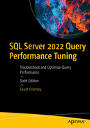
An execution plan highlights the flow of index seek to nested loops and key lookup points compute scalar and finally to the nested loops.
Execution plan for the query showing a key lookup
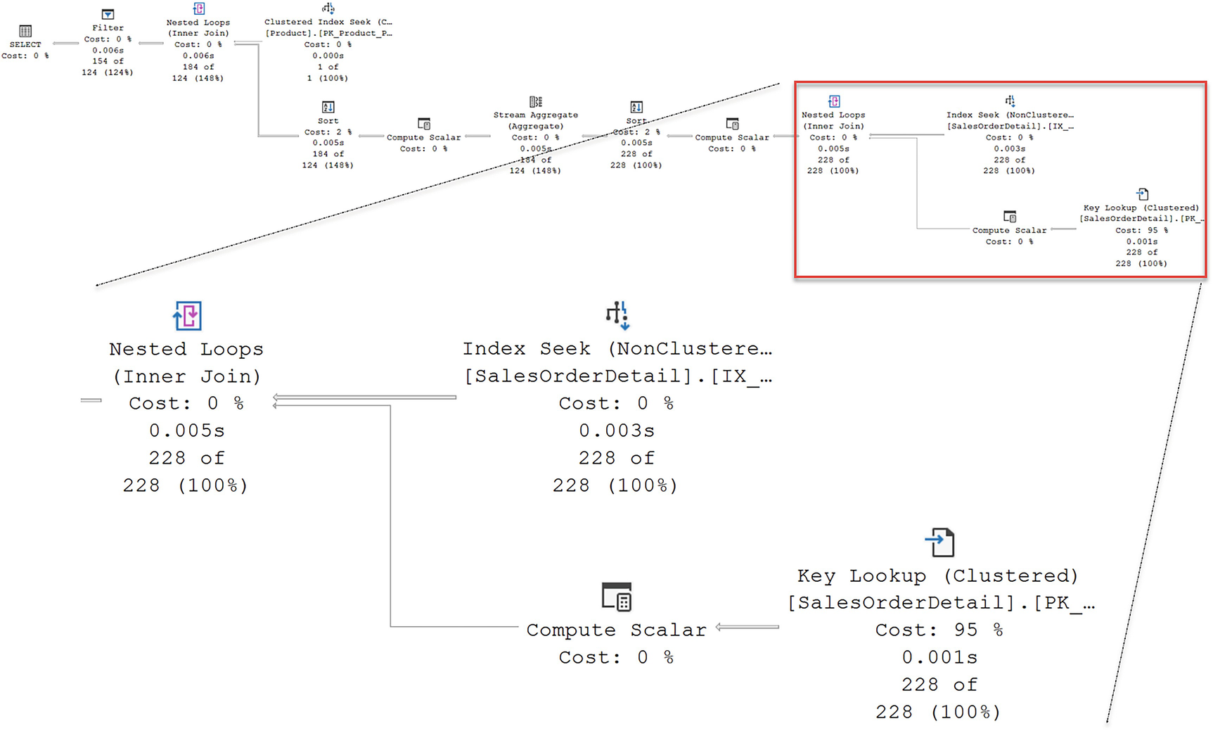
A table with 2 columns and 4 rows. It contains 4 output lists, and the row entries are adventure works, sales, sales order details of a carrier tracking number, order quantity, unit price, and discount.
The Output List property showing the columns in the lookup
Performance Issues Caused by Lookups
A lookup necessitates retrieving pages from where the data is stored as well as the pages from the nonclustered index. Accessing more pages quite simply increases the number of logical reads for a given query. Additionally, if the pages are not available in memory, a lookup will probably require a random (nonsequential) I/O operation on the disk to go from the index page to the data page. On top of that, there is CPU processing necessary to marshal the data and perform the operations.
In addition to that cost, you also add the cost of the join operation necessary to put the two sets of data together.
These costs associated with lookups are why it’s recommended to keep data retrieval from nonclustered indexes to small sets of data. As the data set size increases, the costs associated with lookups go up as well.
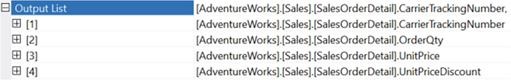
A larger data set from the SalesOrderDetail table
A diagram displays the flow of the clustered index scan that undergoes 2 compute scalar states, filter cost, then select cost.
A scan in order to retrieve a larger data set
Forcing an index to be used
This query will change the plan to one with an index seek and a key lookup, similar to what we saw earlier in Figure 11-1. However, the reads for the query in Listing 11-3 went to 2,251 from the value of 1,248 for Listing 11-2.
As you can see, while the lookup operation is a necessary one, it can be quite costly.
Analysis of the Causes of Lookups
Not all lookups have to be eliminated because some queries aren’t called very frequently and they run fast enough as they are. However, when a query needs to run faster, and there’s a lookup operation, depending on the number of columns that have to be dealt with, that lookup can be some low-hanging fruit to improve performance.
Retrieving basic information from the Employee table
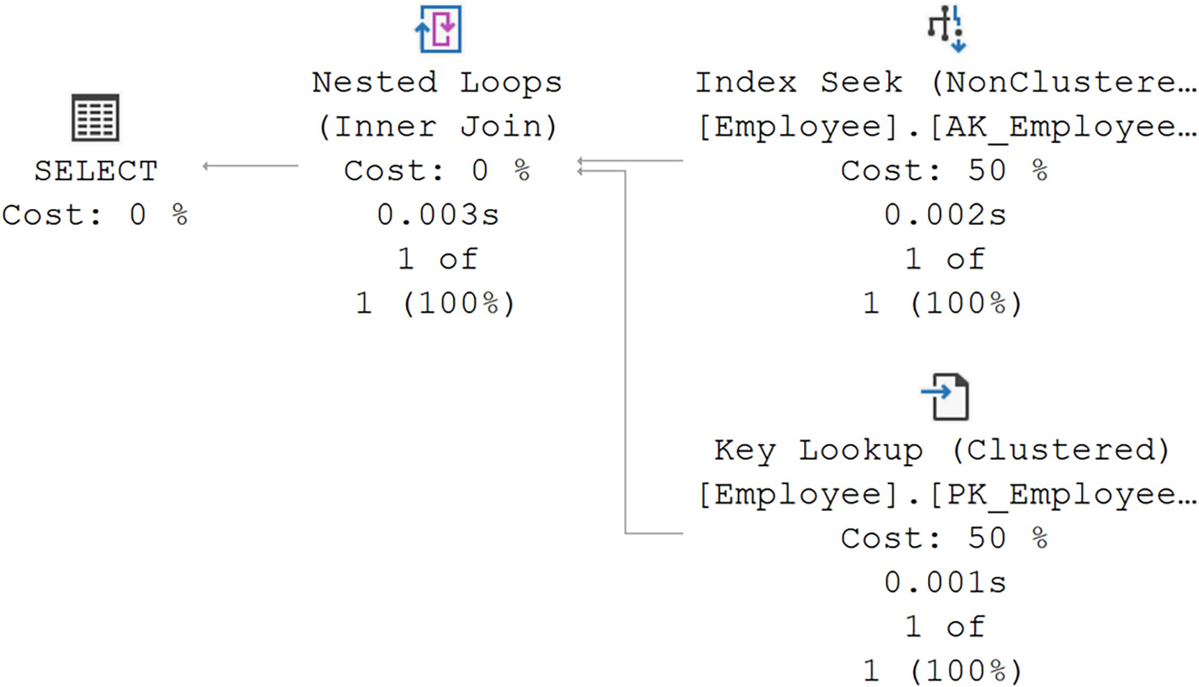
A diagram displays the standard key lookup operation where both indexes seek and key lookup point to nested loops, then point to select.
A standard key lookup operation
In the example in Listing 11-4, since we’re only retrieving three columns from the table, and we know the index is on the NationalIDNumber column, it’s pretty easy to infer that the lookup is for the other two columns. However, with large queries, columns in use in multiple clauses, it can be tricky to simply look at a query and understand which columns you need to deal with.

A table displays the 2 columns of 2 sets of output lists. The output list has an alias, column, database, scheme, and tables.
The two columns in the Output List of the Key Lookup operator

A dialog box of output list with 2 entries. Entries are adventure works, human resources employee job title, and hire date.
Columns highlighted in a text window
With this information, you can now decide how you plan to resolve the lookup operation.
Techniques to Resolve Lookups
I’ve said it already in this chapter, but it bears repeating, not every lookup operation requires immediate attention. Understanding how the query in question is working within the system can help you decide if you need to fix the lookup. However, you’re usually unaware of lookups in queries that are running fast enough. You’re looking at the execution plan of a query because it’s running slowly.
Create a clustered index.
Use a covering index.
Take advantage of index joins.
Let’s explore all three of these in a little more detail.
Create a Clustered Index
Since the leaf pages of a clustered index contain all the columns for a table (with a few exceptions), when a clustered index is used to retrieve the rows, no lookup operations are needed. If the index used for Listing 11-4 earlier was recreated as the clustered index for the table, no lookup operation would occur.
In most cases, this just isn’t an option. You’ve already designed the table around a good, clustered index. You can’t—in fact, you shouldn’t—simply swap those indexes around. At least, not without extensive testing. However, if you’re working with a heap table, you have the opportunity to create a new clustered index, which would resolve any RID lookup operations.
Use a Covering Index
In Chapter 10, I explained that a covering index is one that has all the columns needed to satisfy a given query. This means that the index would not need to go to where the data is stored in order to retrieve all the columns.
Using DBCC SHOW_STATISTICS to see the density graph
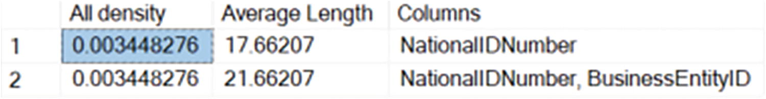
A table displays 3 columns and 2 rows. The column headers are all density, average length, and columns. The first row entry, 0.003448276, is highlighted.
Density graph for the original index
The average key length for the existing index, which includes the indexed column, NationalIDNumber, and the row identifier, in this case, the clustered index key, BusinessEntityID, is 21.66.
Recreating the index with a new key
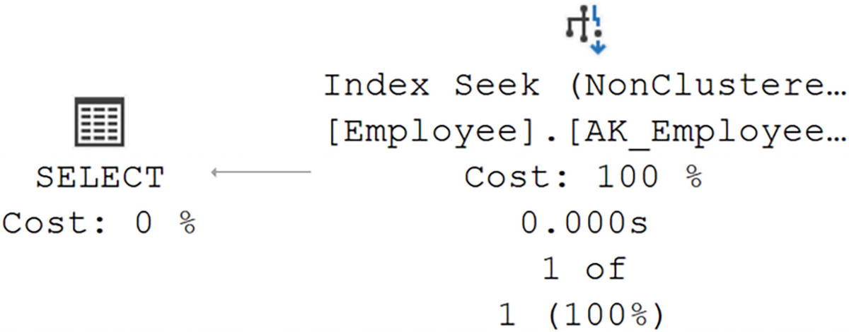
A diagram depicts that the index seeks of non cluster with a cost of 100 percentage points to select.
Lookup operation eliminated
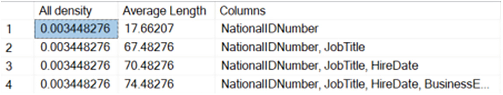
A table has 3 columns and 4 rows. The column headers are all density, average length, and columns. The first column entry, 0.003448276, is highlighted.
The density graph for the new index
The average length of the key has gone from 21.66 to 74.48, more than three times bigger. That means fewer rows per page, and so page reads will go up when accessing this new index. That doesn’t even address the fact that the index behavior is now going to be different overall.
Using the INCLUDE clause to recreate the index

A table has 3 columns and 2 rows. The column headers are all density, average length, and columns. All density values are 0.003448276 and 0.003448276.
Average key length is back down
The average key length is back to what it was because while we’ve added data to the index, it’s stored at the leaf, not on with the key. Overall, this should perform better in terms of reads, although for such a small key and data set, you’re unlikely to see it here in this example.
Resetting the index
A modified query
Once more, this results in an execution plan that looks like Figure 11-8. It’s a covering index because the clustered index key, BusinessEntityID, is included with the index as the row locator. So we can modify code to make an index covering. However, to be fair, we’ve changed the result set. If you need the columns in question, JobTitle and HireDate, this is a horrible solution.
Take Advantage of Index Joins
Query against the PurchaseOrderHeader table
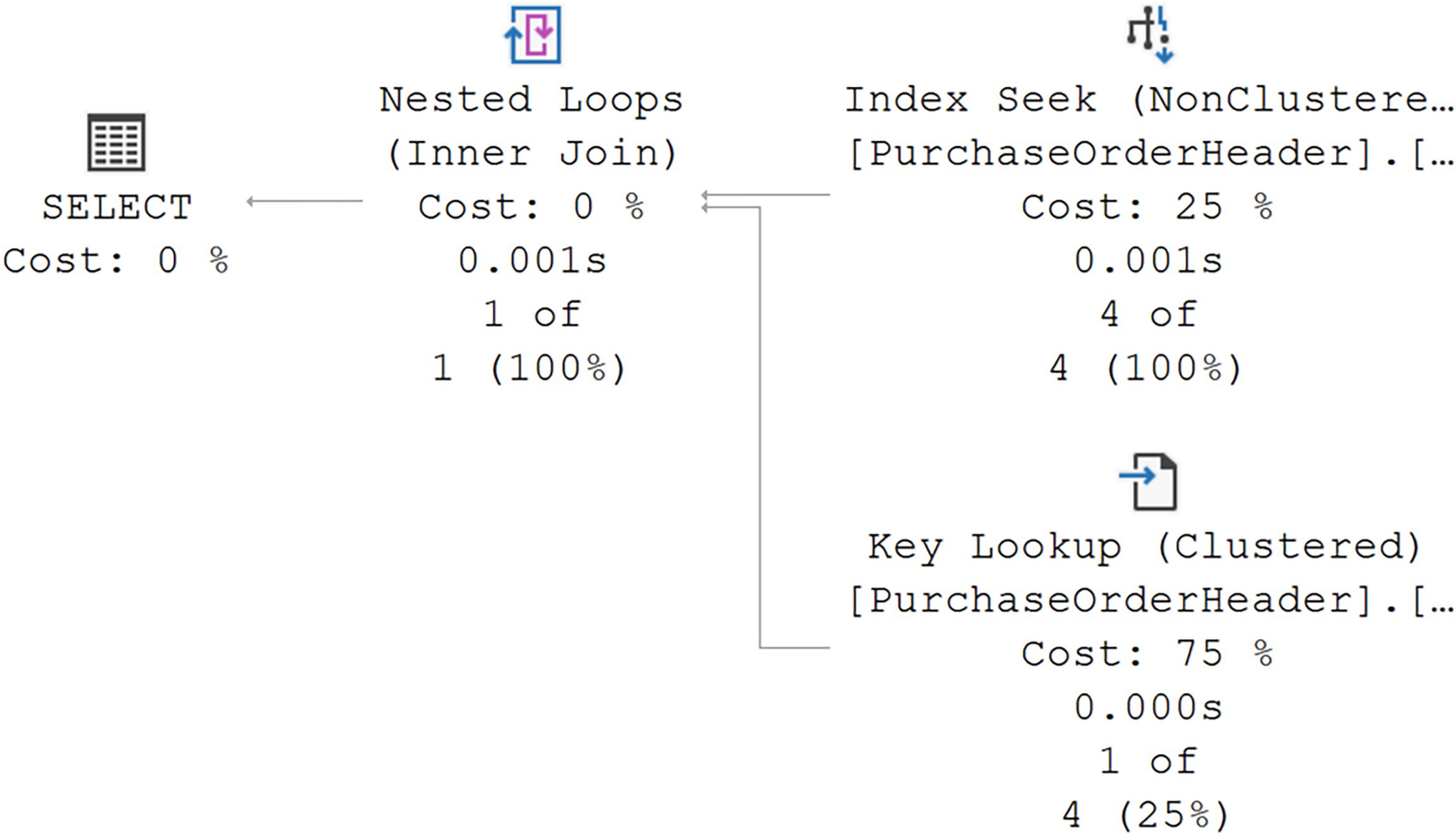
A diagram depicts both index seek and key lookup with costs of 25 and 75 percent, points to nested loops. Then points to select, both with 0 percent cost.
Query resulted in a key lookup
As with the other queries in this chapter, the columns in the query are not contained in any of the nonclustered indexes on the table. This means that even though the IX_PurchaseOrderHeader_VendorID index filters the data based on the WHERE criteria, the rest of the columns in the query have to be retrieved from the clustered index.
As we’ve shown earlier, you could modify the index and add columns to make it a covering index. However, that does change the index, either the key or just the overall size with columns at the leaf level. What if modifying the existing index negatively impacted other queries?
Creating a new nonclustered index
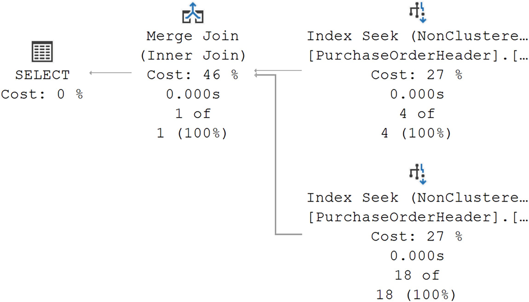
A diagram of a flow of 2 indexes seeks 4 of 4 and 18 of 18, with a cost of 27 percent, to merge join as an inner join, with a cost of 46 percent. Then points to select, with a cost of 0 percent.
An index join works as a covering index
In the execution plan, both indexes are used to seek against. Because the data is ordered in both seek operations, a merge join is used to put together the one matching row. The reads went from 10 to 4, and you saw a similar improvement in performance.
Changing the index IX_PurchaseOrderHeader_VendorID to be covering would perform even better than this, since it eliminates the join operation as well as the reads against the second index. However, as we discussed, we’re avoiding it in this case.
Summary
As you can see from the code and examples in this chapter, there are mechanisms for dealing with lookups, whether a heap or a clustered index. Lookup operations are not free, so they can be a good choice to help improve the performance of a given query. Analyzing the lookup itself is easy since the lookup operation tells you what you need to know. Then it’s just a question of picking one of the possible solutions to fix the issue.
In the next chapter, we’re going to discuss a somewhat controversial topic: index fragmentation. We’ll talk about whether or not fragmentation is a problem and if it becomes a problem, how best to deal with it.