Choosing the correct index can be one of the single most effective mechanisms for enhancing performance within SQL Server. Because of this simple fact, it’s vital that you understand how indexes work in order to help you select the correct one for the job. Back in SQL Server 2016, the Clustered Columnstore index was introduced. Today, we actually get to pick our best storage mechanism for the data, whether a Clustered Rowstore or a Clustered Columnstore index, for the most common data access. Then we can add additional indexes to each to assist other query paths to the data.
What is an index
Recommendations for choosing an index
Clustered and nonclustered rowstore index behavior
Clustered and nonclustered columnstore index behavior
Recommendations on index use
What Is a Rowstore Index?
The existence of an index on a table can be the difference between looking at every single row on the table, in what’s called a scan, and simply going right to the row of information you need. To say that this helps performance, especially I/O, would be a gross understatement. A good analogy for an index in a database is the index in this book. For example, if you were interested in the term parameter sniffing, without an index in the book, you’d have to look at every single page. With the index, you can go directly to the page you need. In the same way, an index in the database takes you right to the information you need.
Retrieving all Products ordered by Name

A screenshot depicts the output. The data includes Product ID, name, standard cost, weight, and row number. Data is ordered by product name.
Data ordered and numbered by Product.Name
You can think about this result set as if it were an index. The data is sorted and stored by Name. You can look up the data by the RowNumber value. In the database, the query shown previously scanned all the data in the table because there is no WHERE clause.
If we were interested in filtering our data and the business requirement was to return only those values where the StandardCost is greater than 200, we’d have to scan the entire table, comparing the values, to determine if a given row exceeded that value. We can take a couple of approaches to create an “index” on this data.

A screenshot depicts the output. The data includes Product ID, name, standard cost, weight, and row number. Date is ordered by standard cost.
Data reordered by StandardCost
Note, I left the sort on the RowNumber value by Name, so you see the original values there.
Finding the values that are greater than 200 would be a simple matter of going to the first value that’s above that and then returning the rest. An index that sorts the data, and stores in that sorted fashion, is a clustered index. Because SQL Server is oriented around the storage of clustered indexes, this is the single most important index to pick in your systems. I’ll explain even more later in the chapter.
An “index” on the StandardCost column
StandardCost | RowNumber |
|---|---|
2171.2942 | 125 |
2171.2942 | 126 |
2171.2942 | 127 |
2171.2942 | 128 |
2171.2942 | 129 |
1912.1544 | 170 |
A structure like this is similar to a nonclustered index. We have a pointer back to the data, in the form of the RowNumber, which would be the primary key on a clustered index, or a row ID in a heap (more about heaps a little later). Again, the value for StandardCost acts as a guide to the value we’re interested in, and then the data is stored with the clustered index.
Hash: Part of the memory optimized table structure, covered in Chapter 20
Memory Optimized Nonclustered: Another part of the memory optimized table structure, also covered in Chapter 20
Spatial: Indexes that work with geometry or geography data in order to optimize search and retrieval of spatial objects, covered in Chapter 10
XML: Indexes for the XML data type, covered in Chapter 10
Full-Text: Indexes built and maintained by the Full-Text Engine within SQL Server, also covered in Chapter 10
The Benefits of Indexes
In order for SQL Server to actually be useful, you need to be able to retrieve the data stored in it. When you have no clustered index defined on a table, the storage engine will be left with no choice but to read through the entire table to find information. A table that has no clustered index is called a heap. A heap is just an unordered stack of data with a row identifier as a pointer to the storage location. The only way to search through the data in a heap is going row by row in a process called a scan. When creating a clustered index, the data itself is reordered and stored by the key you define for that index. The key becomes the pointer to the data, as well as the ordering mechanism. A nonclustered index, as described previously will have a pointer back to the data, either consisting of the RID to a heap or the key to the clustered index. So the first benefit of indexes is the fact that the data is ordered, making it easier to search.
Data within SQL Server is stored on an 8KB page. A page is the minimum amount of information that moves from the disk into memory. How much data you can store on a given page becomes very important for this reason. Generally speaking, a nonclustered index is going to be small, consisting of the key column, or columns, and any INCLUDE columns that you add. Because of this, retrieving data from a nonclustered index means more rows on a page. This makes for better performance because you have to move fewer pages off of disk and into memory, depending on the query of course.
Another benefit of a nonclustered index is that it is stored separately from the table. You can even put it onto a different disk entirely, making searches faster.

A layout of the stored data. From left to right, the sequence of numbers is present.
27 rows in a random order stored in pages
To search for the value of 5, SQL Server will have to scan all the rows on all the pages. Even the last page could have the value of 5. Because the number of reads depends on the number of pages accessed, nine read operations (retrieving the pages from disk and storing them in memory) will be performed on the table since there is no index.

A layout of the stored data. From left to right, the sequence of numbers is present.
27 rows stored in sorted order on the pages

A B-tree structure includes the root node, branch nodes, and leaf nodes.
27 rows stored in a B-Tree
A B-Tree consists of a starting node (or page) called a root node. It has a number of branch nodes (again, or pages) that are below it. Finally, below them are the leaf nodes (pages, also called interior nodes). The root node stores pointers to the branch nodes. The branch nodes store pointers to the leaf nodes. All values are stored in the leaf nodes. The key values that define our index are kept sorted at all times. The balanced nature of the B-Tree is that each of these nodes will be distributed evenly as shown in Figure 9-5. Each of the leaf nodes is in what is referred to as a doubly linked list, meaning each page points to the page that follows it and the page that preceded it. The doubly linked list means that when scanning the values, you won’t have to go back up the chain of nodes to find the next page.
The B-Tree algorithm minimizes the number of pages accessed, speeding up data retrieval. For the value of 5, you would start at the root node. It’s going to point to the first branch node, because its starting value is 1, which is less than five, while the next page starts at 10, so it can be ignored. The branch node page is read, and here, we find a page that starts at the value of 4, greater than the value of 1 and less than the value of 7. It then goes down and reads the leaf node page, reading through all the rows on the page, to return the value of 5. So it took three reads to find 5. While that sounds like more than 2, remember, it will also only take three reads to find the value of 25.
So indexes put the data into ordered storage to help speed processing. They reduce the number of pages to be accessed, again, increasing performance, and, through the B-Tree, further reduce the number of pages to be accessed, again, increasing performance.
There are a number of other benefits from indexes that we’ll explore throughout the book, from enforcing unique values (which can also help performance) to compressed storage and more. Further, we’ll discuss the benefits of the columnstore index in a section later in the chapter.
Index Overhead
Nothing comes for free. While we get a performance benefit from indexes, there is a cost. A table with an index requires more storage and memory space than an equivalent heap table. Data manipulation queries (INSERT, UPDATE, and DELETE statements) can take longer. More processing time is required to maintain the indexes. This is because, unlike a SELECT statement, data manipulation queries modify the content of a table. If an INSERT statement adds a row to the table, then it also has to add a row in the index structure. Since the data is stored in order, it could mean rearranging data within the pages to get it stored in the correct position. Similar issues arise from UPDATE and DELETE.
There are going to be two things to think about when deciding whether or not to add an index. First, will that index help performance? Next, how much will that index negatively impact performance? You will absolutely want to measure the performance improvements that come with an index. However, you should have the capabilities to also measure its impact. I’ll cover that in some detail in Chapter 22. Your best tool here is Extended Events. However, you’ll also want to use the DMVs that show how indexes behave: sys.dm_db_operational_stats and sys.dm_db_index_usage_stats. The operational stats show the behaviors of the indexes including locks and I/O. The usage stats give you statistics counts of index operations over time. I’ll cover these in more detail in Chapter 17.
Most of the measurements I show throughout the book are done using Extended Events as outlined in Chapter 3. However, for some detailed situations, I will use STATISTICS IO and STATISTICS TIME. However, using both of these together in some situations can cause problems. The time it takes to retrieve and transmit the IO data gets added to the time data, making it less accurate. This is why unless I need the object level measurement of IO, I stick to Extended Events.
Building a table with 10,000 rows
Updating IndexTest table
Creating a clustered index on IndexTest
The reads go up because the data has to be reordered in the index. That’s more work than just making the change to the row within the heap table.
A worktable is a temporary table used internally by SQL Server to process the immediate results of a query. Worktables are created in tempdb and are dropped automatically after execution. In this case, the worktable was for sorting the data.
While there is overhead associated with maintaining indexes as data changes, it’s important to remember that SQL Server must find the row in order to update or delete it. This means even while a given data manipulation query may experience overhead due to the index being there, it also gets the benefits of the index in locating the correct row. Frequently, the performance benefit here outweighs the cost.
Creating a new index on IndexTest
We’ve taken the reads from 42 down to 20. That’s even fewer reads than the original heap table, at 29. All because the index helped us more quickly identify which row to modify from our query. While there is certainly overhead to indexes, there are, with equal certainty, benefits to indexes.
What Is a Columnstore Index?
Simply put, a columnstore index stores data by columns instead of by rows. By pivoting the storage of the information, the columnstore index becomes extremely useful when working with analytical style queries. These are queries with a lot of aggregations and counts. Because the data is stored at the column, instead of the row, aggregations are extremely fast because you don’t have to access a large number of rows. You also see benefits because you’re only retrieving data from the columns you want, instead of rows full of columns, some of which you don’t want. You’ll also see performance benefits from columnstore indexes because the data is stored there in a compressed manner by default (you can add compression to rowstore indexes, and I’ll discuss that in Chapter 10).
Some data types cannot be used such as binary, test, varchar(MAX), clr, or XML.
You can’t create a columnstore index on a sparse column.
A table with a clustered columnstore index cannot have constraints, including primary and foreign keys.
Prior to SQL Server 2016, nonclustered indexes cannot be updated.
Columnstore indexes are designed to work best with larger data sets, above 100,000 rows. You can see some benefits on smaller data sets, but not always.
Because AdventureWorks doesn’t have large-scale tables, I’m going to use Adam Machanic’s script, make_big_adventure.sql, to create large tables: dbo.bigTransactionHistory and dbo.bigProduct. The script is available for download from here: Thinking Big (Adventure) - Data Education.
Columnstore Index Storage
I’ve already said it in this chapter, but it bears repeating. Because we now have both rowstore and columnstore clustered indexes, we get to choose data storage that is optimal for the majority of our queries.
Columnstore is not stored in a B-Tree as described earlier. Instead, the data is pivoted and aggregated on each column within the table. Further, the data is broken up into rowgroups. Each rowgroup consists of approximately 102,400 rows (although it’s easier to just think of them as being grouped in sets of 100,000). As data is loaded into a columnstore, it automatically gets broken up into rowgroups.
As data is updated in columnstore indexes, changes are stored in what is called the deltastore. The deltastore is a B-Tree index managed by the SQL Server engine. Added and modified rows are accumulated in the deltastore until there are 102,400 of them. At which point, they will be pivoted, compressed, and stored as a rowgroup.
Deletes from columnstore indexes are not actually immediately removed. Instead, another B-Tree index, again, controlled internally and not visible to the user, tracks a list of identifiers for the rows removed. When the index goes through a rebuild or reorganization, the data is then physically removed.
If you only ever perform batch loads to the columnstore, you really won’t have to worry about the deltastore. However, if you’re doing small batch loads, or a lot of updates, you will be dealing with the deltastore. This is very likely when you have a nonclustered columnstore on a rowstore table. By and large, the deltastore manages itself just fine. However, it’s not a bad idea to rebuild the columnstore index in order to clear out the logically deleted rows and get compressed rowgroups. We’ll cover rebuilds and reorgs in Chapter 11.
The pivoted, grouped, and compressed storage in the columnstore index leads to excellent performance with analytical style queries. However, it’s much slower when performing single row or limited range lookups needed for OLTP style queries.
The overall behavior of a clustered or nonclustered columnstore index is the same. The difference is that the clustered columnstore, like the clustered rowstore, is literally defining data storage for the table. The nonclustered columnstore must have the data stored and managed elsewhere, through either a clustered index or a heap.
Index Design Recommendations
Type of query processing being performed
Determine filtering criteria
Use narrow indexes
Consider the uniqueness of the data
Determine data type
Consider column order
Determine data storage
I’ll discuss each of these in detail in order to help understand what I mean.
Type of Query Processing Being Performed
You first have to determine if your queries are primarily the kind of point lookup and limited range scans commonly associated with an Online Transaction Processing (OLTP) system, or if you are looking at more large-scale data analytic queries involving aggregations. If you are supporting a primarily OLTP system, then you should be looking at rowstore indexes. More specifically, you should be looking at rowstore clustered indexes for data storage. On the other hand, if you are doing a lot of large analytical queries, then you should be focused on columnstore indexes.
Because you can combine each approach using nonclustered rowstore indexes on your clustered columnstore, or using nonclustered columnstore indexes on your clustered rowstore, you should first decide what style the majority of your queries are. After that, you can adjust by adding nonclustered indexes as needed.
Determine Filtering Criteria
Each column used in a WHERE, JOIN, or HAVING clause is identified.
Indexes on these columns are identified.
The usefulness of the index is determined by looking at the selectivity of the index (i.e., the number of rows that would be returned) based on statistics on the index.
If no indexes exist for a column used in filtering, statistics are gathered or created for evaluation.
Constraints such as foreign keys or check constraints are assessed and used by the optimizer.
Finally, the optimizer goes through all this and creates cost estimates for the least costly method of retrieving the matching rows.
Retrieving all data from a table
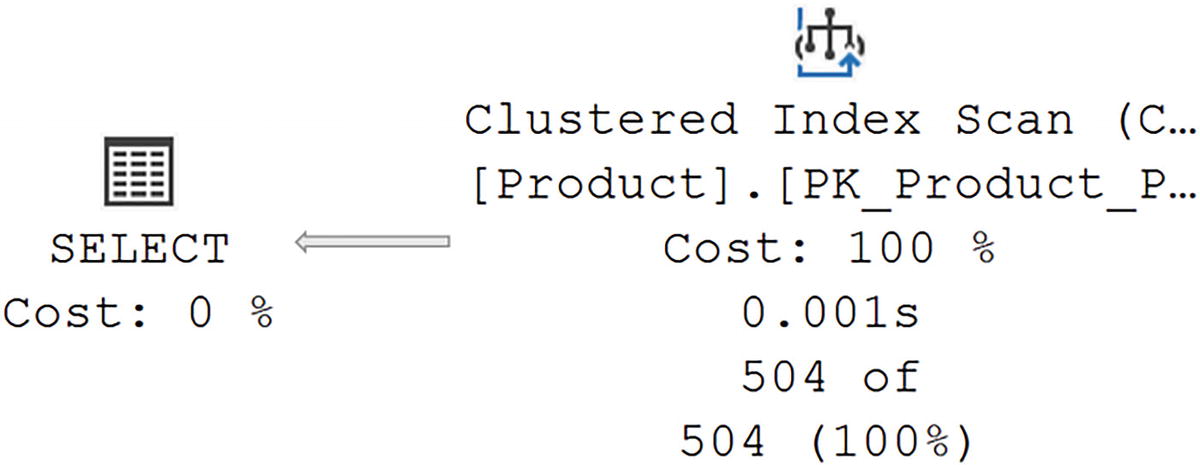
A screenshot represents the execution plan for the clustered index scan to be performed. It includes 100% cost, 0.001 seconds on the right, and on the left a cost of 0%.
A Clustered Index Scan to retrieve all data
Introducing the WHERE clause

A screenshot represents the execution plan for the clustered index seek to be performed. It includes 100% cost, 0.001 seconds on the right, and on the left a cost of 0%.
A Clustered Index Seek because of the WHERE clause
Also, the execution time for the query went from X on average to X.
Don’t forget when measuring execution time, you shouldn’t capture STATISTICS IO or execution plans. Both negatively impact the recorded execution time.
You can see visibly how introducing a WHERE clause gives the optimizer information to work with in making better choices for retrieving data. This is also applicable if you have a JOIN between two tables or a HAVING clause as part of an aggregation. The optimizer could simply scan all tables to retrieve the data. That will work. However, it’s not efficient. The combination of a good index and filtering criteria gets us more efficient data retrieval.
When the amount of data inside a table is so small that it fits on a single page (8KB), you may only ever see a scan. In this case, with such a small amount of data, a scan is every bit as efficient as a seek. In short, you won’t always see a SEEK operation, even if there is a good index in place.
Use Narrow Indexes
To help enhance performance, where possible, use as narrow a data type as is practical. Narrow in this context means as small a data type as you can use. A column defined as an integer (INT) is smaller than a column defined as a variable string, VARCHAR(50). That said, if you need to index on a wider column because that’s how the queries are going to be written, you may have to skip this suggestion.
The reason you should at least consider the possibility is because a narrower key column can fit more rows on your 8KB page, which reduces I/O. You’ll also see improved data caching because fewer pages have to be read into memory.
Creating a test table and index
Getting the size of the index

A screenshot depicts the output. The data includes name, page count, record count, and index level.
Number of pages for a narrow index
I’ve combined a couple of system objects here. First, sys.indexes is a system table, unique to each database, showing all the indexes in that database. I combined it with the DMV to get detailed information about how the index is being stored (I’ll spend more time on how to use the DMV in Chapter 11).
Changing the data type on the existing table

A screenshot depicts the output. The data includes name, page count, record count, and index level.
Number of pages for a wider index
A larger number of pages means more memory use, more I/O, and generally slower performance. You won’t always be able to choose which column to index, but when you can, go for the narrower column.
Consider Selectivity of the Data
Marking an index as unique can enhance performance in multiple ways. The optimizer will know that only a single row can match any given value, or set of values for a compound key; this will change the choices it makes when retrieving the data, but also when performing a join operation as well as other behaviors.
Determining a column’s selectivity
Just change the column and table to run that anywhere.
Retreiving information from the Employee table
Adding an index to the Employee table
Forcing the index use through a query hint

A screenshot represents the execution plan.
Forcing an index seek
Changing the IX_Employee_Test index

A screenshot depicts the execution plan by covering the query. It includes 100% cost, 0.000 seconds, and on the left a cost of 0%.
Index is now covering the query.
Without the need for a query hint (and the modification of the code that requires, unless we forced a hint through Query Store or a plan guide), modifying the index results in a radically faster query and much fewer reads.
As you can see, a more selective index can lead to serious performance improvements.
Removing the test index
Determine Data Type
The data type of an index matters. For example, an index search on integer keys is fast because of the small size and easy arithmetic manipulation of the INTEGER (or INT) data type. You can also use other variations of integer data types (BIGINT, SMALLINT, and TINYINT) for index columns, whereas string data types (CHAR, VARCHAR, NCHAR, and NVARCHAR) require a string match operation, which is usually costlier than an integer match operation.
Suppose you want to create an index on one column and you have two candidate columns—one with an INTEGER data type and the other with a CHAR(4) data type. Even though the size of both data types is 4 bytes in SQL Server 2017 and Azure SQL Database, you should still prefer the INTEGER data type index. Look at arithmetic operations as an example. The value 1 in the CHAR(4) data type is actually stored as 1 followed by three spaces, a combination of the following four bytes: 0x35, 0x20, 0x20, and 0x20. The CPU doesn’t understand how to perform arithmetic operations on this data, and therefore, it converts to an integer data type before the arithmetic operations, whereas the value 1 in an integer data type is saved as 0x00000001. The CPU can easily perform arithmetic operations on this data.
Further, use the correct data type on columns. While you can store numbers in text columns, they’re going to be much bigger than the same number column. An integer stores up to 2,147,483,647 in a 4-byte column. For a VARCHAR to store the same thing, it will have to be 10 bytes in size. That will make for a poor index.
Of course, most of the time, you won’t have the simple choice between identically sized data types, allowing you to choose the more optimal type. Keep this information in mind when designing and building your indexes.
Consider Column Order
An unsorted table
Column1 | Column2 |
|---|---|
1 | 1 |
3 | 1 |
2 | 1 |
3 | 2 |
1 | 2 |
2 | 2 |
A sorted index
Column1 | Column2 |
|---|---|
1 | 1 |
1 | 2 |
2 | 1 |
2 | 2 |
3 | 1 |
3 | 2 |
The data is sorted first on Column1, as the leading edge of the index, and then on Column2.
Creating a new index on the Address table
Querying the Address table

A screenshot depicts the execution plan that uses the index created. It includes 100% cost, 0.000 seconds, and on the left a cost of 0%.
Execution plan that can use the index created
The index provides exactly what the query needs in order to perform quickly. The histogram supplies an accurate row count for the number of rows that are going to be equal to the value of “Dresden”.
A different query for the Address table

A screenshot depicts the execution plan. It includes 100% cost, 0.000 seconds, and on the left a cost of 0%.
The index could not be fully used
We went from 2 reads to 106. It is still using the same test index that we created, but because it’s not looking at the leading edge of the index, it must be scanned to find the matching rows. This also illustrates the power of the covering index, which we’ll cover in Chapter 10.
Dropping the test index
Determine Data Storage
You have to determine how your data is best stored. The storage is driven by the predominant types of queries run against the data. Online Transaction Processing (OLTP) largely consists of smaller sets of data, even single rows. This style of query is best served by rowstore indexes. Analytical queries that aggregate large data sets are best served by columnstore indexes. So first determining how to store your data helps you pick your first index on a given table.
There are additional index types, but we’ll address them in Chapter 10.
Rowstore Index Behavior
The more traditional type of index in SQL Server is the rowstore index. Because of this, I don’t refer to those indexes as “rowstore clustered index” or “rowstore nonclustered index” but instead simply as either a clustered or nonclustered index. However, we do need to take into account that there is more than one way to store and retrieve data, so we’ll approach each in turn, starting with the rowstore indexes.
Clustered Indexes
The data is stored at the leaf level of clustered indexes with the key to the index supplying the order for data storage. Because of this, you get one clustered index per table.
When you create a primary key constraint, by default, it will be a unique clustered index. That is, if a clustered index doesn’t already exist on the table and you don’t specify that this constraint should be nonclustered. While having the primary key be a clustered index is a default behavior, it’s not in any way required. You can choose to make the clustered index on columns other than the primary key.
Heap Tables
A table without a clustered index is referred to as a heap table. The data in a heap is not stored in any kind of order. It’s this unorganized structure that gave it the name heap. As data in a heap grows, more and more overhead is necessary to deal with the unstructured nature of the storage. Except in cases where extensive testing suggests otherwise, it’s best to have a clustered index of some kind on every table in your database.
Relationships with Nonclustered Indexes
A nonclustered index only stores the key values and any INCLUDE values. In order to get at the underlying data, a pointer is stored with the nonclustered index. In the case of a heap table, this is the Row Identifier (RID). In the case of a clustered index, this is the key to the clustered index. The pointer is called a row locator.
Querying the heap table DatabaseLog

A screenshot depicts the execution plan with R I D lookup. It includes 100% cost, 0.000 seconds, and on the left a cost of 0%.
An RID lookup is needed to satisfy the query.
The nonclustered index, the primary key, was helpful to the query as you can see with the Index Seek operation. However, because the data is stored separately, two additional operations are necessary: RID Lookup and Nested Loops. The Nested Loops operator is only there to bring the data together from the other two operations. The RID Lookup is the optimizer going to the heap to retrieve additional data. We’ll go into more on this later in the chapter.
Querying a table stored on a clustered index

A screenshot depicts the execution plan without a lookup. It includes 100% cost, 0.000 seconds, and on the left a cost of 0%.
No lookup required on this query
The query in Listing 9-21 against the heap used the primary key to find the correct row but then had to look up the remaining data. The query in Listing 9-22 used the primary key to find the correct row; then, because the data is stored with the key, no additional operations were needed to satisfy the query.
To navigate from a nonclustered index row to a data row, this relationship between the two index types requires an additional indirection for navigating the B-Tree structure of the clustered index. Without the clustered index, the row locator of the nonclustered index would be able to navigate directly from the nonclustered index row to the data row in the base heap table. The presence of the clustered index causes the navigation from the nonclustered index row to the data row to go through the B-Tree structure of the clustered index, since the new row locator values point to the clustered index key.
On the other hand, consider inserting an intermediate row in the clustered index key order or expanding the content of an intermediate row. For example, imagine a clustered index table containing four rows per page, with clustered index column values of 1, 2, 4, and 5. Adding a new row in the table with the clustered index value 3 will require space in the page between values 2 and 4. If enough space is not available in that position, a page split will occur on the data page (or clustered index leaf page). Even though the data page split will cause relocation of the data rows, the nonclustered index row locator values need not be updated. These row locators continue to point to the same logical key values of the clustered index key, even though the data rows have physically moved to a different location. In the case of a data page split, the row locators of the nonclustered indexes need not be updated. This is an important point since tables often have a large number of nonclustered indexes.
Things don’t work the same way for heap tables. While page splits in a heap are not a common occurrence, and when heaps do split, they don’t rearrange locations in the same way as clustered indexes, you can have rows move in a heap, usually due to updates causing the heap to not fit on its current page. Anything that causes the location of rows to be moved in a heap will result in a forwarding record being placed into the original location pointing to that new location, necessitating even more I/O activity.
Clustered Index Recommendations
The general behavior of the clustered index and its relationship to nonclustered indexes means you should take a few things into consideration when working with clustered indexes.
Create the Clustered Index First
Since all nonclustered indexes contain the clustered index key within their rows, the order of creation for nonclustered and clustered indexes is important from a performance standpoint. For example, if the nonclustered indexes are built on a table before the clustered index, all the row locators are going to the RID of the heap table. Creating the clustered index will then entail recreating all the nonclustered indexes because they need to have the key values replace the RID as row locator.
I recommend you create the clustered index before you create nonclustered indexes. This won’t affect most operations, but it will require additional work, adding to the overhead on the system during the creation process.
As part of creating the clustered index, I also suggest you design the tables in your OLTP database around that index. It should be the first index created because you should be storing your data as a clustered index by default.
I’ll address data warehouse and analytical style queries in the columnstore section later in this chapter.
Keep Clustered Indexes Narrow
Because all nonclustered indexes must carry the clustered index key values, for best performance, keep the size of the clustered index key as small as possible. If you create a wide clustered index, for example, CHAR(500), in addition to having fewer rows per page in the cluster, you will have fewer rows per page in every nonclustered index as 500 bytes gets added to them.
Keep the number, data type, and size of the clustered index keys in mind when designing them. This doesn’t mean if the correct key is wider than other possible columns, you should not use that key. No, please, do use the appropriate key. Simply look for opportunities to use a better key structure where possible.
Queries to create clustered and non-clustered indexes
Getting the size of the indexes on the test table

A screenshot depicts the output. The data includes name, page count, record count, and index level.
The size of indexes with a narrow key
Adjusting the size of the column

A screenshot depicts the output. The data includes name, page count, record count, and index level.
Wider indexes mean more pages
Just those small changes, with small data sets, result in significantly more pages being used. Therefore, a wide clustered key has ramifications beyond its own storage.
Rebuild the Clustered Index in a Single Step
Because of the dependency of nonclustered indexes on the clustered index, rebuilding the clustered index as two statements, DROP INDEX and CREATE INDEX, causes all nonclustered indexes to get rebuilt two times. To avoid this, use WITH DROP_EXISTING as part of the CREATE INDEX statement. That results in a single atomic step and impacts the nonclustered indexes only once.
Where Possible, Make the Clustered Index Unique
Because the clustered index defines data storage, each distinct row has to be identified separately. When the clustered index is a unique value, each row is then identified through that value. However, when the clustered index is not unique, SQL Server must add a value to the index key in order to make it unique. This is called the uniquifier. The uniquifier consists of what is, to all intents and purposes, an IDENTITY column added to your index key. It adds a little overhead to storage and processing for that index, 4 bytes per row to be exact. It’s also possible to run out of uniquifier values (although this is relatively rare). For these reasons, where possible, define the clustered index as unique.
When to Use a Clustered Index
Clustered indexes are best used in a couple of scenarios. However, remember, one of the driving factors for a clustered index is that it’s not just a retrieval mechanism. The clustered index also defines storage of the data.
Accessing the Data Directly
Since all columns for the table are stored at the leaf level of the clustered index, this should be the most common path to the data. When the data is directly retrieved from the clustered index without intervening steps, performance is generally enhanced. When you get into performing lookup operations to get data after the rows have been identified, you are adding overhead to the system.
It bears repeating, frequently, the most common access path to the data is through the primary key of the table, hence why so many are clustered. There may be other columns in the table that would make for a better access path.
The clustered index works well when you’re retrieving data from the table. If you’re retrieving only a small subset of that data, only a few columns, a nonclustered index can become more useful.
If the majority of your queries are analytical in nature, you may be better off using the clustered columnstore index.
Retrieving Presorted Data
Clustered indexes are useful when the data retrieval needs to be sorted (a covering nonclustered index is also good for this). If the clustered index exists on the columns that you need to sort by, then the rows will be physically stored in that order, eliminating the overhead of sorting the data after it is retrieved.
Building the od table from the PurchaseOrderDetail table
Retrieving a large range of rows
Creating a clustered index on the table
We’ve cut the execution time almost in half and reduced the reads from 100 to 30. Having the data stored in order makes the query faster.
Poor Design Practices for a Clustered Index
Clustered indexes are extremely important within SQL Server. However, there are situations where you can negatively impact performance on clustered indexes.
Frequently Updated Columns
If the columns that define the key of the clustered index are frequently updated, this has a direct performance impact. Since the key columns act as the row identifier for nonclustered indexes, each of these nonclustered indexes has to be updated along with the clustered index. That adds quite a bit of additional resource use and will cause blocking as other queries will wait until the data update is complete.
Updating the key on the Sales.SpecialOfferProduct table
Adding a nonclustered index to the SpecialOfferProduct table
You can see that we went from 15 reads to 19, just because additional work has to be done on the nonclustered index.
Dropping the ixTest index
Wide Keys
I’ve already talked about this earlier in the chapter. A wider clustered key means fewer rows per page in the nonclustered index. Where possible, keep the size on your key columns down.
Nonclustered Indexes
The core concept with a nonclustered index is a mechanism to add more ways to sort the data, making more possibilities for retrieving the data. A nonclustered index doesn’t affect the order of the data in the table pages because it’s storing its information separately from the rest of the table. A pointer (row locator) is required to navigate from a nonclustered index to the actual data row, whether on a heap or a clustered index. For a heap, the row locator is the RID for the data row. With a clustered index, the key columns from the clustered index act as the row locator. When you have a nonclustered index on a clustered columnstore index, an 8-byte value consisting of the columnstore’s row_group_id and an offset value make up the row locator.
Nonclustered Index Maintenance
In a table that is a heap, where there is no clustered index, to optimize this maintenance cost, SQL Server adds a pointer to the old data page to point to the new data page after a page split, instead of updating the row locator of all the relevant nonclustered indexes. Although this reduces the maintenance cost of the nonclustered indexes, it increases the navigation cost from the nonclustered index row to the data row within the heap, since an extra link is added between the old data page and the new data page. Therefore, having a clustered index as the row locator decreases this overhead associated with the nonclustered index.
When a table is a clustered columnstore index, the storage values of exactly what information is stored where changes as the index is rebuilt and data moves from the deltastore into compressed storage. This would lead to all sorts of issues except a new bit of functionality within the clustered columnstore index allows for a mapping between where the nonclustered index thought the value was and where it actually is. Funny enough, this is called the Mapping Index. Values are added to it as locations of data change within the clustered columnstore. It can slightly slow nonclustered index usage when the table data is contained in a clustered columnstore.
Defining the Lookup Operation
When a query requests columns that are not part of the nonclustered index chosen by the optimizer, a lookup is required. This may be a key lookup when going against a clustered index, columnstore or not, or an RID Lookup when performed against a heap. The lookup fetches the corresponding data row from the table by following the row locator value from the index row, requiring a logical read on the data page besides the logical read on the index page and a join operation to put the data together in a common output. However, if all the columns required by the query are available in the index itself, then access to the data page is not required. This is known as a covering index.
These lookups are the reason that large result sets are better served with a clustered index. A clustered index doesn’t require a lookup since the leaf pages and data pages for a clustered index are the same. I’ll go over lookups in a lot more detail in Chapter 11.
Nonclustered Index Recommendations
Nonclustered indexes are meant to offer flexibility for your data retrieval. While you only get one clustered index, you can have multiple nonclustered indexes, although it’s a good idea to keep these as minimal as possible since they do come with maintenance overhead.
When to Use a Nonclustered Index
A nonclustered index is most useful when all you want to do is retrieve a small number of rows and columns from a large table. As the number of columns to be retrieved increases, the ability to have a covering index decreases. Then, if you’re also retrieving a large number of rows, the overhead cost of any lookup rises proportionately. To retrieve a small number of rows from a table, the indexed column should have a high selectivity.
Furthermore, there will be indexing requirements that won’t be suitable for a clustered index, as explained in the “Clustered Indexes” section:
Frequently updatable columns
Wide keys
In these cases, you can use a nonclustered index since, unlike a clustered index, it doesn’t affect other indexes in the table. A nonclustered index on a frequently updatable column isn’t as costly as having a clustered index on that column. The UPDATE operation on a nonclustered index is limited to the base table and the nonclustered index. It doesn’t affect any other nonclustered indexes on the table. Similarly, a nonclustered index on a wide column (or set of columns) doesn’t increase the size of any other index, unlike that with a clustered index. However, remain cautious, even while creating a nonclustered index on a highly updatable column or a wide column (or set of columns), since this can increase the cost of action queries, as explained earlier in the chapter.
When Not to Use a Nonclustered Index
Nonclustered indexes are not suitable for queries that retrieve a large number of rows. Such queries are better served with a clustered index, which doesn’t require a separate lookup to retrieve a data row. Since a lookup requires additional logical reads to get to the data page besides the logical read on the nonclustered index page, the cost of a query using a nonclustered index increases significantly for a large number of rows, such as when in a loop join that requires one lookup after another. The SQL Server query optimizer takes this cost into effect and accordingly can discard the nonclustered index when retrieving a large result set. Nonclustered indexes are also not as useful as columnstore indexes for analytics style queries with more aggregates.
If your requirement is to retrieve a large result set from a table, then having a nonclustered index on the filter criterion (or the join criterion) column will probably not be useful unless you use a special type of nonclustered index called a covering index. I describe this index type in detail in Chapter 10.
Columnstore Index Behavior
Aggregate query against BigAdventure tables

A screenshot depicts the execution plan without column store indexes.
Execution plan for an aggregate query without columnstore indexes
Creating the first columnstore index

A screenshot depicts the execution plan with column store indexes.
Columnstore indexes in an execution plan
The execution time was 540ms on average.
Just to emphasize this, we’ve gone from 8.4 seconds on the Linux container running SQL Server 2022 on my laptop to return 24,975 rows to 540 milliseconds. Ignoring the change in the reads, that’s a 15 times increase in speed.

A screenshot depicts the column store index scan.
Columnstore Index Scan of bigTransactionHistory
This is a new operator introduced just for columnstore indexes. It reveals a number of functions internally. Also, this is the first execution plan in the book to have gone into parallel execution. You can tell that a plan is parallel by the addition of those two yellow arrows indicating that a given operation is being done through parallel processing. Parallel processing takes advantage of the fact that you have more than one CPU on a system in order to split up the work done between processors. We’ll cover parallel execution in several places throughout the book.

A screenshot depicts the execution mode and the number of batches.
Batch mode processing and the number of Batches
Batch mode processing was introduced along with columnstore indexes. It’s a much faster way to process the data than with row mode processing. Row mode processing worked through execution plans, a row at a time, passing the rows between operators. Batch mode processing operates on approximately 1,000 rows at a time. In fact, you can see in Figure 9-21 that the Columnstore Index Scan operated as batch mode and that there were 37,422 batches. There were 30,794,071 rows processed. Doing the math, that comes out to about 822 rows per batch.
Prior to SQL Server 2019, batch mode processing was only available to columnstore indexes. Starting in SQL Server 2019, rowstore indexes can also benefit from batch mode processing. We’ll see that in Chapter 10.

A screenshot depicts the properties and the number of batches. It includes locally aggregated rows and rows of all executions.
Showing the Locally Aggregated Rows
The property Actual Number of Locally Aggregated Rows shows that 469,530 rows were aggregated as the data was retrieved. This behavior is yet another enhancement on performance in the columnstore index in support of analytical queries.
It’s generally a good practice to put any column that you’re likely to query against into the columnstore index. It’s not like creating a key in a rowstore index.
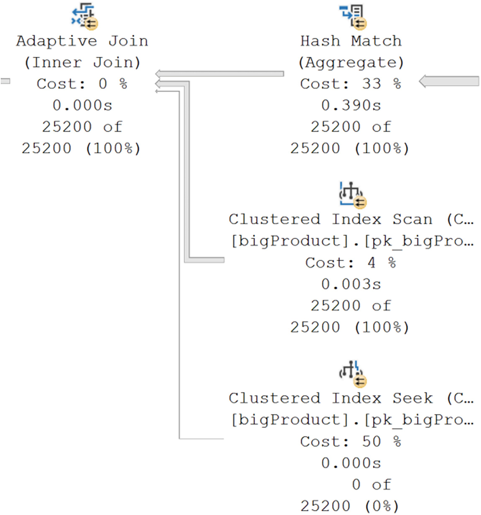
A screenshot depicts the execution plan with clustered index scan and clustered index seek.
The Adaptive Join operator
We’ll be talking about join types throughout the book, as we have already. The Adaptive Join is part of the new automated tuning mechanisms that we’ll cover in detail in Chapter 21. For larger data sets, the Nested Loops join can perform poorly. For smaller data sets, a Hash Join can also perform poorly. The Adaptive Join establishes a data threshold based on the statistics available from the objects involved in the query. Below that threshold, a Nested Loops join will be used. Above that threshold, a Hash Join will be used.

A screenshot depicts the properties of the adaptive join operator and the number of batches.
Properties of the Adaptive Join operator
I’d like to point out several properties here. First, and most importantly, I have highlighted the Adaptive Threshold Rows property. The value is 1,961.3. That means as soon as 1,962 rows are passed to the Adaptive Join operator, it will choose the Hash Join branch. Since 25,200 rows were processed, as we see on the Actual Number of Rows for All Executions property, we have exceeded that value. You can also see at the bottom of Figure 9-24 the Estimated Join Type has a value of HashMatch. That shows the optimizer assumed the number of rows processed was likely to exceed the threshold. You can also see the Actual Join Type, which also has a value of HashMatch. This means you can reliably know which branch was chosen by the Adaptive Join without just looking at row counts. Finally, as a side note, at the top of Figure 9-24, you can see that this operator was also performing in Batch mode.
One other point from this query and the resulting execution plan, you can mix and match columnstore and rowstore indexes and tables in a single query. The optimizer will make appropriate choices for each.
Columnstore Recommendations
It bears repeating, columnstore indexes are best for large-scale, analytical style queries. If you have a more OLTP set of queries, rowstore indexes will serve you well.
Because you can add nonclustered rowstore indexes to a clustered columnstore and you can add nonclustered columnstore indexes to a clustered rowstore, you can deal with exceptional situations in either direction. While you will gain the most benefit from columnstore indexes when you exceed the 102,400-row rowgroup threshold, smaller tables may still get some benefit, depending on the style of queries. Test your system to know for sure.
Load the data into the columnstore in either a single transaction or in batches that are greater than 102,400 in order to take advantage of compressed rowgroups.
Where possible, minimize small-scale updates within columnstore in order to avoid the overhead of dealing with the deltastore.
Plan to have an index rebuild for both clustered and nonclustered columnstore indexes in order to eliminate delete data completely from the rowgroups and move modified data from the deltastore into the rowgroups.
Maintain the statistics on your columnstore indexes similar to how you do the same on your rowstore indexes. While they are not visible in the same way as rowstore indexes, they still must be maintained.
Summary
In this chapter, I introduced the two major types of indexes: rowstore and columnstore. I also walked you through the importance of understanding how your data is being queried in order to help you choose the correct storage mechanism for the data. We explored the strengths and weaknesses of each of the different index types and how they work together to support you storing and retrieving your data in an efficient manner. Finally, we explored how these different index types affect query performance, both positively and negatively.
In the next chapter, we’re going to continue to explore indexes. We’ll look at several modifications you can make to index behavior and some of the special types of indexes available.