While a healthy amount of performance is determined by your hardware, your cloud service tier, server settings, indexes, and other data structures, the single most important aspect of SQL Server performance is your queries. If your T-SQL is problematic, in many cases, none of the rest of functionality can save performance. There are a number of common coding issues, referred to as code smells, that can lead to bad performance. You may even have queries attempting to work on your data in a row-by-row fashion (quoting Jeff Moden, Row By Agonizing Row, abbreviated to RBAR). Focusing on fixing your T-SQL can be the single most important thing you can do to enhance the performance of your databases.
Common code smells in T-SQL
Query designs to ensure effective index use
Appropriate use of optimizer hints
How database constraints affect performance
Query Design Recommendations
Keep your result sets as small as possible.
Use indexes effectively.
Use optimizer hints sparingly.
Maintain and enforce referential integrity.
While all of my recommendations are tested, situationally they may not work for your queries or your environment. You should always make it a habit to test and validate code changes as you make them. Use the information put forward so far within the book, from capturing query metrics to reading execution plans, in order to understand how your own queries are performing.
Keep Your Result Sets Small
Move only the data you need and only when you need to move it.
Limit the columns in your SELECT list.
Filter your data through a WHERE clause.
It’s very common to hear someone say that the business requirement is to return 100,000 rows for a report. Yet if you drill down on this requirement, you may find that they simply need an aggregate, or some other subset of the data. Humans simply do not process 100,000 rows on their own. Be sure you’re only moving the data you need.
Limit the Columns in Your SELECT List
Query with a limited column list
An illustration of the execution plan. The index seeks of non clustered with a cost of 100 percentage points to select with a cost of 0 percent.
An execution plan showing a covering index in action

An illustration of the execution plan. The index seeks of non clustered and key loops of clustered with a cost of 50 percentage points to nested loops and finally to select with a cost of 0 percent.
The query no longer has a covering index
I’m no longer getting the benefit of a covering index. The extra work required to both perform a Key Lookup to get the columns from the clustered index and then the Nested Loops to join the two result sets together ends up doubling the number of reads, from 2 to 4. The query duration on average went up more than five times.
In short, only choose the columns you need at the moment.
Filter Your Data Through a WHERE Clause
In order to see benefits from an index on queries that involve looking up data, and this includes UPDATE and DELETE when they’re finding the data being modified, INSERT when a referential integrity check occurs, and, of course, all SELECT statements, a WHERE clause must be used. Further, as explained in Chapter 8, the selectivity of the column, or columns, referenced in the WHERE, ON, and HAVING clauses determines how that index is used. As much as possible, your queries should be filtering data through these clauses. Where possible, you want to use the most selective column as well.
The majority of applications are going to be working off of limited result sets. While you may need to perform data movement involving all, or just a very large subset, of the data, generally speaking, you should be seeing mostly small data sets being retrieved. The exception of course is analytical queries, but you can better support queries of that type through columnstore indexes. In the event that you are in a situation where you regularly have to move extremely large result sets, you may need to look to external processes and hardware to improve performance.
Use Indexes Effectively
Use effective search conditions.
Avoid operations on columns in WHERE, ON, and HAVING clauses.
Use care in creating custom scalar UDFs.
I’ll break down these guidelines in the following sections.
Use Effective Search Conditions
Search conditions within a WHERE, ON, or HAVING clause can use a very large number of logical operations. Some of those operations are highly effective in allowing the query to work with indexes and statistics. Other operations are not as effective and can actively prevent the efficient use of indexes. Traditionally, we refer to the effective operations as being “Search ARGument ABLE” or sargable for short.
While the use of sargable conditions is in the HAVING, ON, and WHERE clauses, rather than saying all three every time, I’m going to simply reference the WHERE clause. Assume I mean all three when I reference just the one.
There are a few search conditions, introduced in more recent versions of SQL Server, for which these rules don’t exactly apply. For example, SOME/ANY and ALL are dependent on the subquery that defines them. If you use a non-sargable condition in that subquery, then you’ll have issues.
Common sargable and non-sargable search conditions
Type | Search Conditions |
|---|---|
Sargable | Inclusion conditions =, >, >=, <, <=, and BETWEEN, and some LIKE conditions such as LIKE ‘<literal>%’ |
Non-sargable | Exclusion conditions <>, !=, !>, !<, NOT EXISTS, NOT IN, NOT LIKE, and some LIKE conditions such as ‘%<literal>’ or ‘%<literal>%’ |
The non-sargable conditions listed will prevent good index use by the optimizer. Instead of a seek, you’re much more likely to see scans when using these conditions. This is especially true to the logical NOT operators such as <>, !=, and NOT LIKE. Using these will always result in a scan of all rows to identify those that match.
Where you can, implement workarounds for these non-sargable search conditions to improve performance. In some cases, it may be possible to rewrite the logic of a query to use inclusion instead of exclusion operations. You will have to experiment with different mechanisms in order to determine which are going to work in a given situation. Also, don’t forget that additional filtering could limit the scans necessary when multiple columns from one table are in a WHERE clause. Testing is your friend when you have to deal with these types of situations.
BETWEEN vs. IN/OR
A query using an IN condition
A query using an OR condition
A query using a BETWEEN condition

A diagram of execution plans for 3 queries. The clustered index seeks of clustered with a cost of 100 percent, then points to select with a cost of 0 percent.
Three visually identical execution plans
Using IN
Using OR
Using BETWEEN

An illustration of 3 panels of difference between top and bottom plans. 1, Two execution plans of clustered index seek points to select. 2 and 3, a top and bottom plan with properties.
Differences between two execution plans
First, the optimizer has chosen to apply simple parameterization to this query as you can see in the @1 and @2 values within the second predicate. Also, instead of a BETWEEN operation, >= and <= have been substituted. In the end, this approach results in far fewer reads. On a production system under load, this will doubtless lead to superior performance.
For the OR query:
For the BETWEEN query:
As you can see, there are four scans to satisfy the OR condition, while a single scan satisfies the BETWEEN condition.
This is not to say that you will always see better performance under all circumstances between IN, OR, and BETWEEN. However, as you can tell, while three queries may share logical similarities, choosing different mechanisms can arrive at superior performance. Testing, and then using the tools to evaluate the queries, is the key. Different operators can, and will, use the indexes in different ways.
This is also an example where STATISTICS IO can give us additional information beyond what’s available to us within Extended Events. You won’t always need to use it, but keep that tool in mind when you need to drill down to better understand why you may be seeing differences in behavior between two queries.
LIKE Condition
Using the LIKE condition
The change is from a LIKE condition to >= and < conditions. You could rewrite the query to use those conditions yourself. If you did, the performance, including the reads, would be exactly the same. This simply means using leading characters in a LIKE condition means the optimizer can optimize the search using indexes on the table.
!< Condition vs. >= Condition
Even though both !< and >= are logically equivalent and you will see an identical result set in a query using them, the optimizer is going to implement execution plans differently using these two conditions. The key is in the equality operator for >=. That gives the optimizer a solid starting point for using an index. The other operation, !<, has no starting point, resulting in the entire index, or the entire table, having to be scanned.
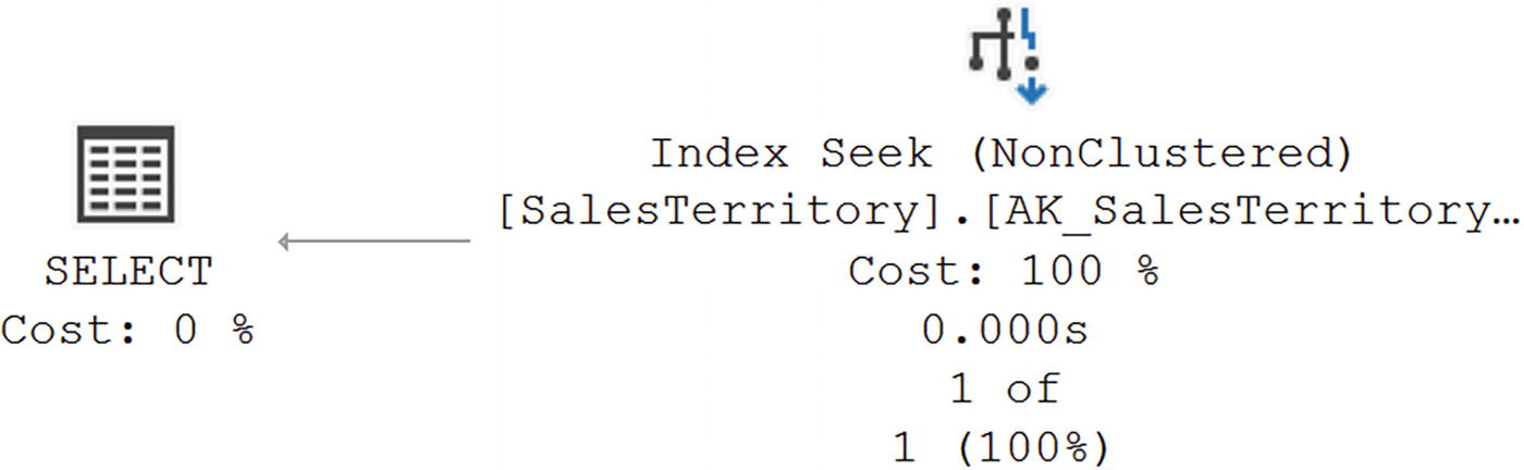
Comparing !< and >= conditions
An execution plan of two queries. Both queries with a clustered index seek points to compute scalar, which has a cost of 1 percent, and finally to select.
Identical execution plans
In fact, if you compare the plans, they are identical. It’s the same execution plan, used for both queries. You can see what happened if you look at the T-SQL stored with the plan. First, the optimizer changed the !< to >=. Second, it used simple parameterization, which leads to plan reuse. This is an example of when code is logically equivalent, the optimizer can help the performance of your query.
Avoid Operations on Columns
Calculation on a column

A diagram displays index scan and key lookup with costs, 67 and 18 percent point to nested loops, with cost 15 percent, then points at select with 0 percent cost.
An index scan caused by a calculation
There is an index on the PurchaseOrderID column, so the optimizer scanned that instead of scanning the clustered index. This is because the nonclustered index is smaller. However, that scan results in the need to then pull the remaining columns from the clustered key through the Key Lookup operation and a join.
In Listing 14-8, I move the calculation off the column to the hard-coded value.
Changing the query to not calculate on the column

A diagram depicts a clustered index seek, with a cost of 100 percent, points at select with a cost of 0 percent.
A seek with the calculation removed
There’s not much to explain. Because of the calculation, the optimizer must scan the data. The optimizer tries to help you by scanning a smaller index and then looking up the remaining data, but as you can see, simply moving the calculation off the column makes all the difference.
Creating an index on a DATETIME column
Querying for parts of dates
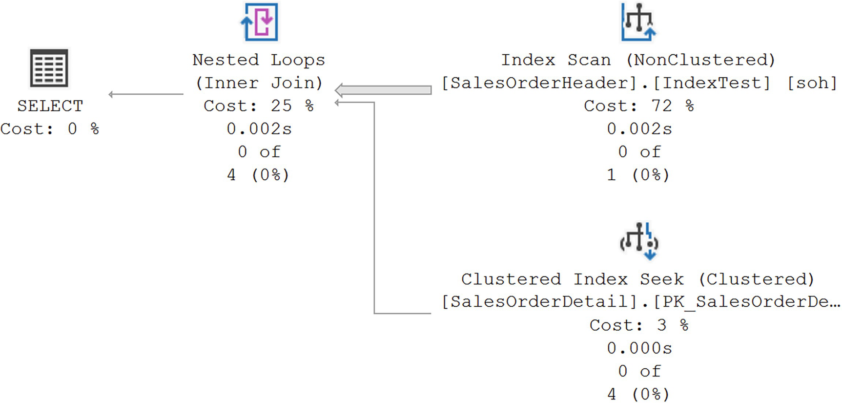
A diagram of the execution plan with index scan and clustered index seek points to nested loops. Finally, from nested loops to select with a cost of 0.
An index scan caused by the DATEPART function
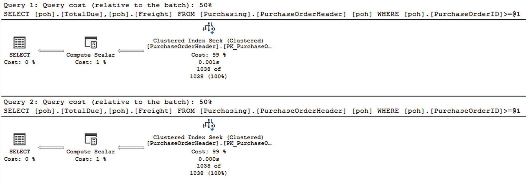
Modifying the date logic

A diagram of the index seeks, and clustered index seek, with the cost at 50 percent, points to nested loops with 0 percent cost. Finally, points at select with 0 percent cost.
A seek occurs when dates are treated appropriately
It’s not even close. In both examples, changing the logic to avoid running operations against columns results in radical performance enhancements.
Cleaning up after the test
Custom Scalar UDF
Scalar function to retrieve product costs
Consuming the scalar function

A diagram execution plan with a scalar function. It includes the connections of clustered index seek, the index seeks to nested loops, compute scalar, and select.
Execution plan with a scalar function
This is a hard-to-read execution plan, so we’ll break it down into its component parts. Older versions of SQL Server won’t show this level of detail within the execution plan but instead will hide the scalar function within a single Compute Scalar operator. Capturing an Estimated Plan will show all the information you see here.
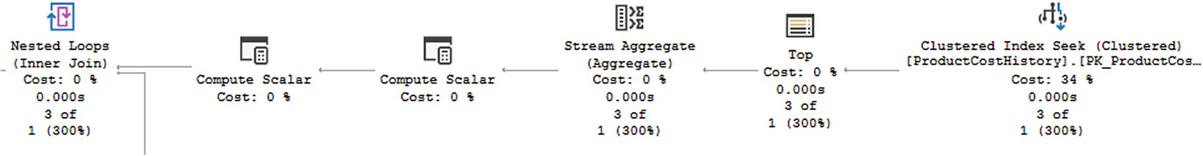
A diagram depicts the data retrieval from the clustered index seek, top cost, stream aggregate, 2 compute scalars, then finally to nested loops.
Data retrieval inside the scalar function
The function is able to use a Clustered Index Seek to retrieve the data. You can then see it performs the necessary functions to prep the information, using a Top operator to support the TOP 1 part of the query and a Stream Aggregate to define the value returns. The Compute Scalar operators just ensure that the data types are correct.

A diagram of the execution plan has 2 constant scan that points to nested loops with a cost of 0 percent.
IF statement within the execution plan
The Constant Scan operators are used to evaluate whether or not the @Cost value is NULL. The join operation will ensure that a value, either the @Cost value or the value of 0, gets returned. This is then joined to the output of the data retrieval in the scalar operator.

A diagram of satisfying the rest of the query. It contains index seeks and key lookup that points to 2 nested loops, then computes scalar. Finally, points to select with a cost of 0 percent.
Satisfying the rest of the query
The Index Seek filters the data from the WHERE clause, and then the Name column is retrieved using the Key Lookup. This data is then joined and then joined again with the data from the scalar function.
Replacing the scalar function

A diagram of index seeks and key lookup that points to 2 nested loops. The clustered index seeks points to the top, then to the second nested loops. Finally, points to select with a cost of 0 percent.
Simplified execution plan after eliminating the scalar function
If you compare this plan to the plan shown previously, you can see most of the same functionality in play. Yet because there are fewer join operations and others, the speed is improved.
Minimize Optimizer Hints
The query optimizer within SQL Server is one of the most amazing pieces of software of which I’m aware. The way it uses your data structures, statistics, and its algorithms to make the queries you write run fast is incredible. However, the optimizer will not always get things perfectly correct, every time. Rarely, it may need some assistance, and you can take some aspects of control away from the optimizer in these cases through the use of what are called hints.
More often than not, the optimizer will give you a good enough plan for the query in question. However, like in the case of parameter sniffing (discussed in Chapter 13), the optimizer’s choices can be less than optimal. As I showed, one way to deal with parameter sniffing gone bad is through the use of a query hint, such as OPTIMIZE FOR. It’s extremely important to understand that a hint is not a suggestion nearly as much as it’s a command for the optimizer to behave in a certain way. The majority of the time, I reserve hints to the very last option when attempting to improve the performance of a query. However, understanding what hints are and how they can be used when you need them is also important.
I don’t have room in the book to cover all possible hints. I have already covered some in earlier chapters, and I’ll cover more in later chapters. Here, I want to demonstrate two specific hints: JOIN hint and INDEX hint.
JOIN Hint
JOIN types supported by SQL Server
JOIN Types | Index on Joining Columns | Usual Size of Joining Tables | Sorted Data Requirement |
|---|---|---|---|
Nested Loops | Inner table a mustOuter table preferable | Small | Optional |
Merge | Both tables a must | Large | Yes |
Hash | Inner table not indexed | Any | No |
Adaptive | Uses either Hash or Loops, so those requirements are needed | Generally, very large | Depends on the join type |
JOIN hints
JOIN Type | JOIN Hint |
|---|---|
Nested Loops | LOOP |
Merge | MERGE |
Hash | HASH |
REMOTE |
There are four hints, but only three JOIN types because the REMOTE hint is used only when one of the tables in a JOIN is in a different database.
Joining multiple tables in a query

A diagram depicts the index seeks and key lookup that points to a hash match, then to a nested loop. The clustered index seeks points to nested loops. Then nested loop points to compute scalar and finally select.
Execution for a query without any hints
Adding a JOIN hint

A diagram of the clustered index scan and clustered index seek points to 2 nested loops. The clustered index seeks points to second nested loops. Then nested loop points to compute scalar and finally to select.
Plan after forcing LOOPS joins
Forcing just one join to behave a certain way

A diagram depicts that the clustered index scan points to sort, nested loops, merge join, nested loops, compute scalar, and select. The clustered index seeks points to nested loops. The clustered index seeks points to merge join, and clustered index seeks points to second nested loops.
Forcing a single join to change may have consequences
Cause elimination of simplification
Prevent auto-parameterization
Prevent the optimizer from dynamically deciding the join order
While hints can sometimes improve performance, it’s absolutely not a guarantee. Only use them after very thorough testing.
INDEX Hints
Forcing index choice through a query hint

A diagram of a scan from an index hint. The cluster index scan with a cost of 100 percentage points to select, which has a cost of 0 percent.
A scan from an index hint
This is a mixed result. The reads went from 11 to 44. However, the execution time went from 2.5ms to 682mcs, a very substantial reduction. It’s still not as fast as simply removing the calculation from the column, which ran in 142mcs and only had 2 reads. Fixing the code is absolutely the superior choice by every measure. However, the INDEX hint did help the original query. This kind of experimentation can sometimes result in wins.
Using Domain and Referential Integrity
While the primary purpose of domain and referential integrity is to ensure good, clean data, the optimizer can also take advantage of these constraints. Knowing that a foreign key is enforced can change the row estimates and improve the choices made by the optimizer.
The NOT NULL constraint
A check constraint
Declarative referential integrity (DRI)
NOT NULL Constraint
The NOT NULL constraint ensures that a given column will never allow NULL values, helping ensure domain integrity of the data there. SQL Server will enforce this constraint in real time as data is manipulated within the table. The optimizer uses the information that there will be no NULL values to help improve the speed of the queries against the column.
Querying the Person.Person table

A diagram of two queries. Index scan of non clustered with a cost of 100 percentage points to select with a cost of 0 percent.
Two visually identical execution plans
The key difference is visible in the plan. The first query is returning 18,967 rows out of an estimated 18,942. The second is returning 11,134 out of 11,372. That’s about the only real difference. Because neither the FirstName nor the MiddleName column has an index to support these queries, a scan of the IX_Person_LastName_FirstName_MiddleName index is used.
Fixing the logic of the second query
Adding indexes to make the queries faster

A diagram of two queries. 1, index seek points to select. 2, three constant scan points to three compute scalar, then concatenation, compute scalar, sort, merge interval. Merge interval and index seek points to nested loops, then finally select.
Indexes and IS NULL changed the execution plans
The first query against the FirstName column used the new index to simply retrieve the data. While the second query was able to use the new index, because of the IS NULL operation, you can see that the plan has greatly expanded in scope in order to satisfy that criterion. Three values are created using the three Constant Scan and Compute Scalar operators, one for each criterion in the WHERE clause. These are then sorted and merged and used in a join to arrive at the filtered data set.
An interesting point worth noting is that the first execution plan has a higher estimated cost. This is meaningless since the queries and data sets are different. However, there is some accuracy here as the first query runs in about 14.5ms while the second runs in 9.6ms.
This is a place where experimenting with using a filtered index to deal with the NOT NULL may result in a performance enhancement. In this case, it actually doesn’t. There are more reads and a slightly slower performance when making TestIndex1 a filtered index. One other point worth bringing up about NULL values is that you can use Sparse columns. This helps reduce the overhead and space associated with storing NULL values. It’s handy for analytical data when you have a lot of NULLs. However, it comes at a performance overhead, so generally it is not considered to be a way to enhance query behaviors.
Dropping the test indexes
User-Defined Constraints
Ensuring that the UnitPrice is greater than zero
No rows returned from this query

A diagram depicts a constant scan with 100 percent cost points to select with 0 percent cost.
An execution plan with no data access at all
The Constant Scan operator is simply a placeholder that the optimizer will use in execution plans to build data sets against. However, in this case, there is only the Constant Scan operator. So what’s happening?

A dialog box of Output List. It contains 5 entries, Order date, ship date, order quantity, unit price, and product name, and a close button at the bottom right.
The Output List to produce an empty result set
If the optimizer didn’t make this choice, since there is no index in support of the preceding query, you’d get a Clustered Index Scan, reading all the data in the table, but returning zero rows. The optimizer saved us from a nasty performance hit because it can read the constraints.
The optimizer can only use a check constraint if it was created using the WITH CHECK option. Otherwise, the constraint is untrusted because the data hasn’t been validated.
Declarative Referential Integrity
Declarative referential integrity (DRI) is the most used mechanism within SQL Server to ensure data cleanliness between a parent and a child table. DRI ensures that rows in the child table only exist when the corresponding row exists in the parent table. The only exception here is when a child table has NULL values in the column, or columns, that refer back to the parent. In SQL Server, DRI is defined through the use of FOREIGN KEY constraint on the child that matches a PRIMARY KEY or UNIQUE INDEX on the parent.
When DRI is established between two tables and the foreign key columns of the child table are set to NOT NULL, the optimizer is assured that for every row in the child table, a corresponding row exists in the parent table. The optimizer can use this knowledge to improve performance because accessing the parent table isn’t necessary to verify the existence of a row for the corresponding child row.
Removing foreign key constraints
Two nearly identical queries

A diagram of 2 queries with identical execution plans, which consists of 2 clustered index seek, points to nested loop, then to select.
Two identical execution plans
Creating a foreign key constraint on the Address table
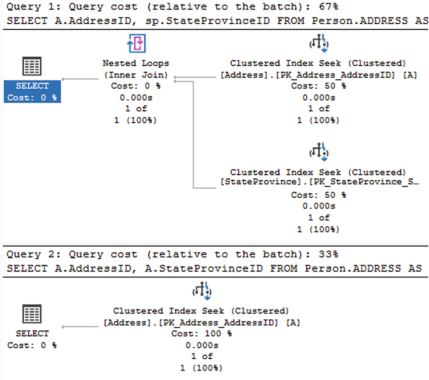
A diagram of execution plans of two queries. 1, Two cluster indexes seek points to nested loops and finally select. 2, cluster index seeks points to select.
The execution plans are now different because of the foreign key
Clearly, the second query now has a new execution plan. When the foreign key wasn’t present, the optimizer didn’t know if rows in the parent and the child table, StateProvince and Address, matched. So it had to validate that by using join operation, Nested Loops in this case. However, with the foreign key put back in place, specifically using the WITH CHECK option to validate the data, the optimizer could now simplify the execution plan and ignore the JOIN operation entirely, arriving at superior performance.
Summary
As important as your structures are, poor decisions with your T-SQL code can hurt performance just as much as if you had never taken the time to create appropriate indexes and maintain your statistics. The optimizer is extremely efficient at working out how best to retrieve your queries, but your queries need to be designed to work with the optimizer. While query hints are available and can be useful, thoroughly testing them before using them is a great practice. Finally, make sure you’re taking advantage of constraints and referential integrity. It’s not only important to make sure that queries are using your structure, but that they avoid excessive resource use.
The next chapter will be focused on reducing resource usage within queries.