Statistics on Rowstore Indexed Columns

The degree to which a given index can help your queries run faster is largely driven by the statistics on the column, or columns, that define the key of the index. The optimizer uses the statistics from the index key columns to make row count estimates, which drive many of the other decisions. SQL Server has two ways of storing indexes: rowstore and columnstore (we’ll be covering them both in Chapter 9). For rowstore indexes, statistics are created automatically along with the index. This behavior cannot be modified. You can add statistics to a columnstore index if you choose. Nonclustered indexes added to columnstore indexes do have statistics because they are still rowstore indexes.

Changes in data can affect index choice. If a table has only one row for a certain column value, then using the index could be a great choice. If the data changes over time and a large number of rows now match that value, it could be that the index becomes less useful. This is why you need to ensure that you have up-to-date statistics.

By default, SQL Server will update statistics on your indexes as the indexed column’s data changes over time. You can disable this behavior if you choose. There is a setting called Auto Update Statistics that can be changed to control this behavior.

In the calculation, “n” represents the number of rows in the table. You’re basically getting the MIN, or minimum, of the two calculations. Let’s assume a larger table with 5 million rows. The first calculation results in a value of 1,000,500. The second calculation results in a value of 70,710. This would then mean that data modifications to only 70,710 rows will result in a statistics update.

With the older method, more than 1,000,500 rows would have to be inserted, updated, or deleted before the statistics would update automatically. As you can see, that would mean a lot fewer updates, therefore, more out-of-date statistics.

You can also make the choice to update statistics asynchronously. Normally, when statistics need to be updated, a query stops and waits, until that update is complete. However, with asynchronous statistics updates, the query will complete, the statistics will update, and then any other queries using those statistics will get the updated values.

You can disable the automatic statistics maintenance using the ALTER DATABASE command. I strongly recommend that you keep this enabled on your systems. Exceedingly few systems suffer from the automatic statistics maintenance, and most systems benefit from it. You can decide to turn on the asynchronous statistics update if you’re seeing timeouts and waits caused by the statistics update.

Benefits of Updated Statistics

Let’s explore how statistics updates benefit query performance. In order to directly control the data in the tables, instead of using AdventureWorks tables for this example, Listing 5-1 will create a table for the test.

DROP TABLE IF EXISTS dbo.Test1;

GO

CREATE TABLE dbo.Test1

(

    C1 INT,

    C2 INT IDENTITY

);

SELECT TOP 1500

       IDENTITY(INT, 1, 1) AS n

INTO #Nums

FROM master.dbo.syscolumns AS sC1,

     master.dbo.syscolumns AS sC2;

INSERT INTO dbo.Test1

(

    C1

)

SELECT n

FROM #Nums;

DROP TABLE #Nums;

CREATE NONCLUSTERED INDEX i1 ON dbo.Test1 (C1);

Listing 5-1

Creating a table and index

We can now run a query against that table that will return one row and use the index as shown in Listing 5-2.

SELECT t.C1,

       t.C2

FROM dbo.Test1 AS t

WHERE t.C1 = 2;

Listing 5-2

Retrieving a single row from the table

We can see the execution plan for the query in Figure 5-1.

A flow diagram exhibits, from right to left, nonclustered index seek and R I D lookup with 50% costs, nested loops with 0%, and select with 0%.

We’re going to use an Extended Events session to watch the behavior of the statistics update processes, as well as capture query performance. Listing 5-3 shows how to set up such a session.

CREATE EVENT SESSION [Statistics]

ON SERVER

    ADD EVENT sqlserver.auto_stats

    (ACTION

     (

         sqlserver.sql_text

     )

     WHERE (sqlserver.database_name = N'AdventureWorks')

    ),

    ADD EVENT sqlserver.sql_batch_completed

    (WHERE (sqlserver.database_name = N'AdventureWorks'));

GO

ALTER EVENT SESSION [Statistics] ON SERVER STATE = START;

Listing 5-3

Creating and starting an Extended Events session

We’re going to add a row to the table (Listing 5-4).

INSERT INTO dbo.Test1

(

    C1

)

VALUES

(2  );

Listing 5-4

Adding a single row to the Test1 table

If we run the SELECT query from Listing 5-2 again, the execution plan is still the same as what we see in Figure 5-1. Figure 5-2 shows the output of the Extended Events session.

A table has name, timestamp, batch text, duration, logical r e, and c p u time columns and 2 rows. The s q l batch completed entry in the second row is highlighted and where an arrowhead points to.

We don’t see any updates from the statistics because adding a single row won’t cross the threshold for statistics updates. Even if it did, just one more row also wouldn’t result in a new execution plan. To understand the effect of data modification on statistics, we’ll add 1,500 rows to the table (Listing 5-5).

SELECT TOP 1500

       IDENTITY(INT, 1, 1) AS n

INTO #Nums

FROM master.dbo.syscolumns AS scl,

     master.dbo.syscolumns AS sC2;

INSERT INTO dbo.Test1

(

    C1

)

SELECT 2

FROM #Nums;

DROP TABLE #Nums;

Listing 5-5

Adding 1,500 rows

Now when we execute the SELECT query from Listing 5-2, we’re going to be retrieving a very large data set, 1,502 rows out of only 3,0001. Since a large result set is being requested, scanning the table directly will be preferable to going to the nonclustered index. This is especially true since the Nested Loops join will require us to access that index 1,501 times. You can see the execution plan resulting from the data changes in Figure 5-3.

A flow diagram exhibits, from right to left, the connection from table scan with 100% cost, 1502 of 1502, to select with 0% cost.

Figure 5-4 shows the resulting output from the Extended Events session.

A table has name, timestamp, batch text, duration, logical r e, statistics list, and status columns and 3 rows. The auto stats entry in the first row is highlighted.

Since we updated so many rows, we exceeded the threshold, so the statistics were updated. I captured the column showing the statistics_list and status from the auto_stats event. You can see that auto_stats was called twice: once, to load and update the dbo.Test.i1 statistics and the second time showing that those statistics were successfully updated. Then, the query ran. The statistics were updated, which resulted in a change to the execution plan. It now has a single table scan instead of 1,501 seek operations. This also illustrates why you want to test carefully if asynchronous statistics updates are desirable. This query could have run with the old execution plan.

Drawbacks of Outdated Statistics

In the previous section, the statistics within SQL Server were automatically updated. The updated statistics are then used to create a new, better, execution plan. That illustrates the advantages of up-to-date statistics. Statistics can become outdated. Then, the optimizer may make poor choices that don’t accurately reflect the data within the system, which will lead to bad performance.

I’m now going to demonstrate what happens when statistics are out of date. To do this, follow these steps:

1. 1.

   Run Listing 5-1 again to recreate the test table with 1,500 rows and the nonclustered index.

    
2. 2.

   Disable automatic statistics updates using Listing 5-6.

    

ALTER DATABASE AdventureWorks SET AUTO_UPDATE_STATISTICS OFF;

Listing 5-6

Disabling automatic update of statistics

1. 3.

   Add 1,500 rows to the table using Listing 5-3.

    

With that setup, we can run the SELECT statement from Listing 5-2, which will result in the execution plan plus runtime metrics shown in Figure 5-5.

A flow diagram exhibits, from right to left, nonclustered index seek and R I D lookup with 40% and 59% costs, nested loops with 0%, and select with 0%.

Because the automatic statistics maintenance has been disabled, the optimizer chose an execution plan based on bad estimates of row counts. You readily see that in the execution plan in Figure 5-5 where the estimated number of rows is 2 and the actual is 1,501, a 75050% variance.

Let’s also look at the differences in the performance metrics of the query. Table 5-3 shows the average duration and the reads of the query with up-to-date statistics and out-of-date statistics.

Table 5-3

Performance measurements of different statistics maintenance

Statistics Update Status	Execution Plan	Avg. Duration (ms)	Number of Reads
Up to date	Figure 5-3	1.6	9
Out of date	Figure 5-5	4.1	1,510

The number of logical reads and the duration are significantly higher with out-of-date statistics. That performance degradation and the difference in the number of reads are despite the fact that we are running the exact same query with the exact same result sets. The differences in how the optimizer satisfies a query, even with everything else being identical, result in serious performance changes. The benefits of keeping statistics up to date usually far outweigh the cost of performing the updates.

Before we finish this section, turn AUTO_UPDATE_STATISTICS back on (Listing 5-7).

ALTER DATABASE AdventureWorks SET AUTO_UPDATE_STATISTICS ON;

Listing 5-7

Enabling automatic statistics update

Statistics on Nonindexed Columns

It’s very common to see columns that are not a part of the index key being used in filtering and join criteria. When this happens, the optimizer still needs to understand the cardinality and data distribution of the column, just like one that has an index on it, in order to make better choices for the execution of the query.

While a column not taking part in an index means that no index exists to help retrieve the data, the optimizer can still use the statistics to create a better plan. This is why, by default, SQL Server will automatically create indexes on columns used for filtering. One scenario where you may consider disabling the automatic creation of statistics is where you are executing a series of ad hoc T-SQL queries that will never be executed again. It’s possible that creating statistics on columns in this scenario could cost more than it benefits you. However, even here, testing to validate how performance is positively or negatively impacted is necessary. For most systems, you should keep the automatic creation of statistics enabled unless you have very clear evidence that the creation of those statistics is actively causing your system pain.

Benefits of Statistics on a Nonindexed Column

To see the benefits of statistics on a column that is not a part of an index, Listing 5-8 will create two test tables with wildly varying data distributions. Both tables contain 10,001 rows. Table Test1 contains only one row for the column, Test1_C2, equal to 1 with the remaining 10,000 rows showing that value as 2. Table Test2 is exactly the opposite data distribution (Listing 5-8).

DROP TABLE IF EXISTS dbo.Test1;

GO

CREATE TABLE dbo.Test1

(

    Test1_C1 INT IDENTITY,

    Test1_C2 INT

);

INSERT INTO dbo.Test1

(

    Test1_C2

)

VALUES

(1  );

SELECT TOP 10000

       IDENTITY(INT, 1, 1) AS n

INTO #Nums

FROM master.dbo.syscolumns AS scl,

     master.dbo.syscolumns AS sC2;

INSERT INTO dbo.Test1

(

    Test1_C2

)

SELECT 2

FROM #Nums;

GO

CREATE CLUSTERED INDEX i1 ON dbo.Test1 (Test1_C1);

--Create second table with 10001 rows, -- but opposite data distribution

IF

(

    SELECT OBJECT_ID('dbo.Test2')

) IS NOT NULL

    DROP TABLE dbo.Test2;

GO

CREATE TABLE dbo.Test2

(

    Test2_C1 INT IDENTITY,

    Test2_C2 INT

);

INSERT INTO dbo.Test2

(

    Test2_C2

)

VALUES

(2  );

INSERT INTO dbo.Test2

(

    Test2_C2

)

SELECT 1

FROM #Nums;

DROP TABLE #Nums;

GO

CREATE CLUSTERED INDEX il ON dbo.Test2 (Test2_C1);

Listing 5-8

Two test tables with varying data distributions

We need to verify that SQL Server is still running with the default statistics creation behavior. We can do that using the DATABASEPROPERTYEX function shown in Listing 5-9.

SELECT DATABASEPROPERTYEX('AdventureWorks2017', 'IsAutoCreateStatistics');

Listing 5-9

Checking database properties using DATABASEPROPERTYEX

The resulting value should be 1. If it’s 0, you’ve disabled the automatic creation of statistics at some point and need to reenable it (Listing 5-10).

ALTER DATABASE AdventureWorks SET AUTO_CREATE_STATISTICS ON;

Listing 5-10

Enabling the automatic creation of statistics

With all that set, we can now test the behavior of statistics on columns that are not a part of an index key. Listing 5-11 shows a SELECT statement that joins our two tables together. A large set of data from Test1 will be returned and a small set of data from Test2 because of the data distribution we have created. Worth noting, the columns used in the join and filter operations have no index on either table.

SELECT t1.Test1_C2,

       t2.Test2_C2

FROM dbo.Test1 AS t1

    JOIN dbo.Test2 AS t2

        ON t1.Test1_C2 = t2.Test2_C2

WHERE t1.Test1_C2 = 2;

Listing 5-11

Joining the two test tables

Figure 5-6 shows the execution plan plus runtime metrics for Listing 5-11.

A flow diagram exhibits, from right to left, tests 2 and 1 of clustered index scans with 27% costs, nested loops with 46%, and select with 0%.

You can see that the pipes estimated data movement correlates with the actual data, very thin for Test2 and much thicker for Test1. After combining the data in the Nested Loops join, the data output pipe is still thick, representing the 10,000 rows being accessed.

Our Extended Events session output shows four auto_stats events, creating the statistics on the columns used in the JOIN and WHERE clauses of the query from Listing 5-11. Figure 5-7 shows the output.

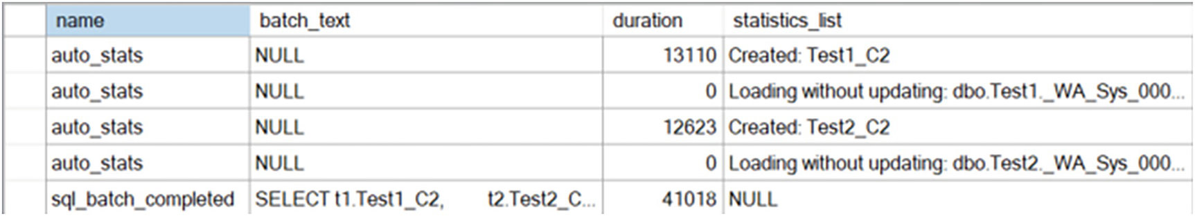
A table has name, batch text, duration, and statistics list columns and row entries of 4 auto stats and 1 s q l batch completed.

You can see in the statistics_list property how the statistics are created on a column and then those statistics loaded for use by the optimizer. To see the statistics created, we run a query against the sys.stats table from Listing 5-12.

SELECT s.name,

       s.auto_created,

       s.user_created

FROM sys.stats AS s

WHERE object_id = OBJECT_ID('Test1');

Listing 5-12

Querying the sys.stats table to see table statistics

You can see the results for the query in Figure 5-8.

A zoomed section of an application exhibits a table with name, auto created, and user created columns and 2 rows under the Results tab. The i 1 entry under name is highlighted.

The auto_created column lets you know that statistics were automatically created with a value of 1. However, you can also see the standard naming convention with “_WA_Sys*” for all automatically created statistics. Of note here is that the statistics for the index, i1, were automatically created along with the index, but they don’t actually count as being auto_created.

We can see the optimizer making different choices based on the statistics if we change the query from Listing 5-11 into the query in Listing 5-13 where we filter on the value 1 instead of 2.

SELECT t1.Test1_C2,

       t2.Test2_C2

FROM dbo.Test1 AS t1

    JOIN dbo.Test2 AS t2

        ON t1.Test1_C2 = t2.Test2_C2

WHERE t1.Test1_C2 = 1;

Listing 5-13

Filtering on different criteria

The resulting execution plan is just a little bit different as you can see in Figure 5-9.

A flow diagram exhibits, from right to left, tests 1 and 2 of clustered index scans with 27% costs, nested loops with 46%, and select with 0%.

If you were to execute the query, you wouldn’t see any auto_stats events since the statistics are already in place. What we do see is that by changing the query, the execution plan has changed. In Figure 5-6, Test2 was the inner table of the Nested Loops join operation. In Figure 5-9, we’ve swapped to Test1 being the inner table. The optimizer can justify this change based on the difference in the data as reflected in the statistics that were automatically created on the columns in question.

Obviously, if we were concerned with improving performance, we’d likely need to add indexes to the columns in question. However, you can see that the optimizer can use statistics on nonindexed columns that will change plan behaviors.

Comparing Performance with Missing Statistics

Just as we saw in the section earlier in the chapter, if the statistics are missing from columns, the optimizer will make less optimal choices. Run Listing 5-8 to recreate our tables without any automatically created statistics. Alternatively, you can identify the names of the automatic statistics and use the DROP STATISTICS command. Either way, we need to disable the automatic creation of statistics using Listing 5-14.

ALTER DATABASE AdventureWorks SET AUTO_CREATE_STATISTICS OFF;

Listing 5-14

Disabling the automatic creation of statistics

The SELECT query in Listing 5-11 will result in the execution plan you see in Figure 5-10.

A flow diagram exhibits select at 0% cost as an endpoint that test 2 of clustered index scan at 22% cost and test 1 of clustered index scan, with respective warnings, with the same cost via a table spool at 20% connects to via an x marked nested loop at 35% costs.

Without statistics, the query optimizer made some very different choices in how it satisfied the query. You can immediately see the warnings on the Clustered Index Scan operations. Here is one of the warnings:

Columns With No Statistics: [AdventureWorks].[dbo].[Test2].Test2_C2

This shouldn’t be a surprise since we reset our table and disabled the ability of SQL Server to create statistics. So the optimizer recognizes that these columns are in use in filtering operations, but without statistics.

The Nested Loops join also has a warning:

No Join Predicate

In short, because there is no way for the operator to estimate row counts, it’s effectively assuming that all values will have to be matched to all values. Because of this, it has chosen a Table Spool, a temporary storage mechanism within execution plans, as a way to store the data read from the Clustered Index Scan against table Test1. By doing this, it thinks it can reduce the number of times it has to scan the table.

Table 5-4 shows the comparison of performance between the two execution plans for the identical query and result set.

Table 5-4

Runtime metrics for two different execution plans

Existence of Statistics	Execution Plan	Avg. Duration (ms)	Number of Reads
With statistics	Figure 5-6	9.6	48
Without statistics	Figure 5-10	37.1	20,244

The number of reads and the duration were much higher on the query without statistics. Because it didn’t have statistics, the optimizer simply made guesses, using mathematical heuristic calculations of course, as to how the data might be distributed. These guesses are simply not as accurate as having actual data for decision-making.

If you do disable the automatic creation of statistics, it might be a very good idea to keep an eye on just how many queries have a need for statistics. Extended Events provides an event called missing_column_statistics.

Header

The Header contains information about the statistics. Some of the data is straightforward such as the Name and the Updated value. The rest is descriptive about the statistics. The Rows column represents the number of rows in the table at the time that the statistics were created or updated. The Rows Sampled column shows how many of the rows were sampled to create the statistics, in this case, 10,001. The header lists how many Steps are in the histogram, here, only 2. The Density is shown as the average key length for the index. The rest of the columns are just describing the state of the statistics in question and are dependent on other settings, which we’ll cover later in the chapter.

Density

The next data set, visible in the middle of Figure 5-11, is the measure of the density. When creating an execution plan, the optimizer analyzes the statistics of columns used in JOIN, HAVING, and WHERE clauses. A filter with high selectivity limits the number of rows that will be retrieved from a table, which helps the optimizer keep the query cost low. A column with a unique index will have a very high selectivity since it limits the number of matching rows to one.

On the other hand, filters with low selectivity will return larger results from the table. A filter with low selectivity can make a nonclustered index ineffective. Navigating through a nonclustered index to the base table for a large result set is less efficient than simply scanning the clustered index (or the base table in the case of a heap).

Statistics track the selectivity of a column in the form of a density ratio. There are two calculations: one for a single column set of statistics like what we’re dealing with here and a second for compound statistics consisting of more than one column. We’ll cover the compound statistics in a later section. The basic calculation is as follows:

Density = 1/Number of distinct values for a column

The results will be the same as those shown in Figure 5-12.

The density is used to estimate the number of rows when the histogram won’t work. The calculation is simple: multiply the density value times the number of rows to get an estimate on the average number of rows for any given distinct value within the table.

Histogram

Figure 5-12 shows a subset of the histogram from these statistics.

A table has unlabeled, range hi key, range rows, e q rows, distinct range rows, and a v g range columns and 13 rows labeled 81 to 93.

So now, let’s assume we have a value, 827. If we look at the RANGE_HI_KEY values, the closest one, above our value, is 831. If we then look over at the AVG_RANGE_ROWS, we get the value 36.66667. If the optimizer were creating an execution plan, it would estimate that there would be 36.66667 rows that matched the value, 827.

Cardinality

This estimate is predicated on the idea that columns of data are related to one another. By getting the power of 1/2 of the selectivity, then 1/4, 1/8, etc., depending on the number of columns involved, the data is treated as if the columns were interrelated, which they usually are.

Another calculation takes effect when dealing with monotonically increasing values, such as an IDENTITY column. With a fresh set of statistics, which have been created using a FULLSCAN (explained later in the “Statistics Maintenance” section), everything simply works as expected. However, if you have used a sampled method to create the statistics, or there have been additions to the table, then the cardinality estimation assumes an average number of rows from the statistics. Prior to SQL Server 2014, the assumption was that all data only returned one row, whether it did or not. The newer method ensures more accurate execution plans in most cases. However, if you have uneven distribution in your data, referred to as skewed data, it can lead to bad cardinality estimations that can result in badly performing execution plans.

You can use Extended Events to observe how cardinality estimations get made. It’s only useful if you really don’t understand where a particular estimate is coming from. Usually that information is easily correlated between the information in the execution plan and the statistics on the columns or indexes. The event in question is query_optimizer_estimate_cardinality.

The first time I run this query, I will generate a number of calls to get cardinality estimation from the optimization process. You can see the output of my Extended Events session in Figure 5-13.

A table with 4 columns and 5 rows with highlighted query optimizer estimate cardinality entry. The details of this event are exhibited as a table with field and value columns and 9 rows.

You can see the auto_stats events firing as they did earlier. Then, highlighted, I have the first query_optimizer_estimate_cardinality event selected, so you can see all the properties of the event at the bottom of the screen. The two areas we have to focus on are the input_relation value and the stats_collected value. Both are XML. The interesting numbers are the Card values. The first is 460.00 (highlighted), showing the overall cardinality of the table, the number of rows. The second value is 1.00, the estimated number of rows from the statistics in question.

Now, we can use this in correlation with the execution plan. Pull the plan from any source, with or without runtime metrics. Then, using the Find Node functionality (described in Chapter 4), we can look for the stats_collection_id value of 38, shown at the bottom of Figure 5-13. That will take us to Node 6 in the plan, the Clustered Index Seek operator against the ProductVendor table. You can see the values in Figure 5-14.

A table has 2 columns and 7 entries. The stats collection I D and 38, as entries on the fifth row, are highlighted.

Again, this is only useful in rare circumstances because, as you can see, the cardinality values are included in the operators. Only if you need to look for obscure issues will this be useful.

Another piece of information returned by this event is the Cardinality Estimation Engine version. This is useful when you’re dealing with upgrades or issues caused by the Cardinality Estimator (we’ll discuss this some more later in the chapter).

This event is not available on Azure SQL Database.

Statistics on a Multicolumn Index

When dealing with an index with a single key column, statistics are defined by the histogram and the density value for that column. When an index has a compound key, more than one column defining the key, then the information is a little different. The histogram stays the same. The first column in a compound key is always the one used to create a histogram. This makes choosing the order of your columns in a key important because only that first column will ever get a histogram, so you want to use the column that has the best data distribution, generally, the most selective column, the one with the lowest density. Then density values include the density for the first column and then for each additional column in the index key. Multiple density values ensure that the optimizer can get more accurate row estimates when multiple columns from the index are used in the predicates of a WHERE, HAVING, or JOIN clause. Here again, column order will matter in the Density calculation as described in the earlier section.

If we run that query, you can see the results in Figure 5-15.

A table has unlabeled, name, auto created, user created, filter definition, column i d, and column name columns and 1 to 8 labeled leftmost row entries under the Results tab. The first entry, P K Product Product I D, under the name column is highlighted.

None of the existing statistics has more than one column. I’m going to run the query from Listing 5-21 and then run the query from Listing 5-22 again. The results are visible in Figure 5-16.

A table has unlabeled, name, auto created, user created, filter definition, column i d, and column name columns and 1 to 10 labeled leftmost row entries under the Results tab. W A sys 0000000 F and 00000006 are added as the last 2 entries.

As you can see, rather than creating a multicolumn set of statistics, one each for each of the columns in question has been added.

Figure 5-17 then shows the statistics that now exist on the index.

3 tables with varying numbers of columns and 1, 2, and 2 rows under the Results tab. First Index, 0.5, and 1 as entries in the first row of each table under the name, all density, and range hi key columns are highlighted.

You can now see that the density has changed to show just the density of the first column and then the density with the addition of the second column. Nothing has changed in the histogram because it’s always, only, on the first column.

Statistics on a Filtered Index

The resulting output from DBCC SHOWSTATISTICS against this new index is shown in Figure 5-18.

3 tables with varying numbers of columns and 1, 2, and 152 rows under the Results tab. I X Test, 0.000262674, and NULL as entries in the first row of each table under the name, all density, and range hi key columns are highlighted.

The updated statistics are visible in Figure 5-19.

3 tables with varying numbers of columns and 1, 2, and 151 rows under the Results tab. The filter expression column with open parenthesis open square bracket purchase order number close square bracket is not null close parenthesis entry is highlighted.

The first thing to note between the information in Figure 5-18 and Figure 5-19 is the number of rows, going from 41,465 to 3,806. You can also see that the key length has increased since we no longer have NULL values. You can also see a Filter Expression for the first time in this chapter. I highlighted it in Figure 5-19.

The density measures are an interesting case. The density is close to the same for both values, but the filtered density is slightly lower, meaning fewer unique values. This is because the filtered data, while marginally less selective, is actually more accurate, eliminating all the empty values that won’t contribute to filtering the data. The density of the second value, which is the clustered index pointer (discussed in Chapter 6), is identical with the value of the density previously because each represents the same amount of unique data. Finally, the histogram shows a NULL value in step 1 in Figure 5-18, but not in Figure 5-19.

You can create filtered statistics as well. Doing this lets you create finely tuned histograms. These are especially useful on partitioned tables. This is necessary because statistics are not automatically created on partitioned tables, and you can’t create your own using CREATE STATISTICS. You can create filtered indexes by partition and get statistics or create filtered statistics specially by partition.

Controlling the Cardinality Estimator

That would make the database behave as if it were a SQL Server 2012 database. This means that much of the more modern behaviors of the database are also disabled. This is generally a poor choice.

It’s much easier to understand what you’re doing and easier to query the behaviors you have set through DATABASE SCOPED CONFIGURATION, available in SQL Server 2016 and greater.

You can also apply trace flag 9481 through a query hint if you choose, or you’re on an older version of SQL Server. It will behave the same way. If you look at the execution plan for the query in Listing 5-29, you can validate which cardinality estimation engine is in use by looking at the properties of the first operator. Find the CardinalityEstimationEngineVersion property as shown in Figure 5-20.

A zoomed section of a table exhibits two entries in one row under two columns that read cardinality estimation model version 70.

And finally, you can use the Query Store hint feature if you’re on SQL Server 2022 or in Azure SQL Database and Azure Managed Instance. We’ll cover the Query Store hint feature in Chapter 6.

Auto Create Statistics

We’ve already discussed how statistics get created on columns without an index when those columns are used as filtering criteria in a JOIN, WHERE, or HAVING clause. This behavior is enabled by default and generally should be left in place.

Auto Update Statistics

We’ve already discussed how statistics get updated. As before, you should leave the defaults in place unless strong testing shows that disabling it on a given system is worth having out-of-date statistics. If you do disable the automatic update of statistics, ensure that you build your own statistics maintenance routines to ensure your statistics are up to date.

Auto Update Statistics Asynchronously

We’ve mentioned this several times in the chapter, but we haven’t yet explained how it works in detail. When Auto Update Statistics Asynchronously is set to on, the basic behavior of statistics in SQL Server isn’t changed radically. When a set of statistics is marked as out of date through the formula established, the statistics update process does not interrupt the execution of the query, like what normally happens. Instead, the query finishes execution using the older set of statistics. Once the query completes, the statistics are updated. This approach can be attractive because when statistics are updated, the current execution plan is removed from cache and a new execution plan is created. Depending on the query in question, creating a new execution plan could be a time-consuming process, delaying the execution of the query. Rather than making a query wait for both the update of the statistics and the generation of the new execution plan, the query completes its run. The next time the same query is called, it will have updated statistics waiting for it, and it will have to recompile only.

Although this functionality does make the steps needed to update statistics and recompile plans faster, it can also cause queries that could benefit immediately from updated statistics and a new execution plan to suffer with the old execution plan. Testing is required before enabling this functionality to ensure it doesn’t cause more harm than good.

Manual Maintenance

Manage Statistics Settings

You can also use the UPDATE STATISTICS command’s WITH NORECOMPUTE option to disable this setting for all or individual indexes and statistics on a table in the current database. The sp_createstats stored procedure also has the NORECOMPUTE option. The NORECOMPUTE option will not disable automatic update of statistics for the database, but it will for a given set of statistics.

Avoid disabling the automatic statistics features, unless you have confirmed through testing that this brings a performance benefit. If the automatic statistics features are disabled, then you are responsible for manually identifying and creating missing statistics on the columns that are not indexed and then keeping the existing statistics up to date. In general, you’re only going to want to disable the automatic statistics features for very large tables.

Create Statistics Manually

You will see a statistics object get created for a columnstore index, but the values inside that set of statistics are null. Individual columns on a columnstore index can have system-generated statistics. When dealing with a columnstore index, if you find you’re still referencing individual columns in filtering queries, it’s possible that creating a multicolumn statistic is useful.

You may find that allowing the automatic updating of statistics is not quite adequate in all circumstances. Scheduling UPDATE STATISTICS for the database during off-hours is a perfectly acceptable way to deal with this issue. UPDATE STATISTICS is the preferred mechanism because it offers a greater degree of flexibility and control. It’s possible, because of the distribution of your data, that the sampling method for gathering statistics may not be accurate enough. The sampled method is the default because it’s faster. However, if you are hitting a case where the statistics aren’t accurately reflecting the data, you can force a FULLSCAN so that all the data is used to update the statistics. This is the same as when a statistic is initially created. FULLSCAN can be a costly operation, so it’s best to be selective about which statistics receive this treatment.

When you create your own statistics, they are treated as a permanent object. As such, they can prevent changes to the table. Automatically created statistics are automatically dropped as needed when tables and indexes are modified. Starting in SQL Server 2022, you can modify the creation of your statistics to include the ability to automatically drop. Simply add WITH AUTO_DROP = ON to the end of the statistics creation. You can also modify statistics to automatically drop by adding the same WITH statement during an UPDATE of statistics.

Resolving a Missing Statistics Issue

Since the index is created on the columns C1 and C2, the statistics on the index contain a histogram for the first column, C1, and density values for the combination of columns (C1 and C1*C2). There are no histograms or density values alone for column C2.

Figure 5-21 shows the resulting execution plan with runtime metrics.

A flow diagram exhibits, from right to left, the connection from test 1 of table scan with 100% cost, with a warning sign, to select with 0% cost.

The first two things to note on the execution plan are the warning and the fact that only three rows were returned, but 5,001 were expected. The warning is letting us know that there is a problem with the Table Scan operation. If we look at the properties page, we’ll find the warning shown in Figure 5-22.

A pop up window labeled Warnings. The text box contains a 1 liner detail for columns with no statistics.

You get a warning when there are no statistics on a column used in a filtering operation because the optimizer knows that it’s not going to be able to ensure accurate row estimates. Between this clear warning and the huge disparity between estimated and actual rows, you know that you’re missing statistics. On average, this query ran in 1.4ms with 88 reads.

If we then run Listing 5-39 again, Figure 5-23 shows the resulting execution plan.

Reads: 34

Duration: 4.9ms

A flow diagram exhibits, from right to left, tests 1 of nonclustered index scan and R I D lookup with 75% and 15% costs, nested loops with 10%, and select with 0%.

Because it now has statistics to work with, the optimizer can accurately estimate that only three rows are going to be returned by the query. Because of this, the optimizer also decides that a better approach would be to use the index iFirstIndex to scan for the data. However, because the index only contains some of the data, we have to go to the table and perform a row lookup using the RID Lookup operation. The number of reads went from 88 to 34, a win. However, because of the extra processing needed for the Nested Loops join and the RID Lookup, the duration actually increased from 1.4ms to 4.9ms, a loss. A fix is possible here. Adding the C3 column as an INCLUDE on the index would result in improved performance. We’ll be covering that sort of solution in later chapters in more detail.

Resolving an Outdated Statistics Issue

Outdated or incorrect statistics are just as damaging as missing statistics. The choices the optimizer makes may be highly inappropriate for the current data distribution. Unfortunately, the execution plan won’t show the same glaring warnings for outdated or incorrect statistics as they do for missing statistics. Instead, you’re going to be looking primarily at the comparison of estimated rows to actual rows in the execution plan.

There is a Debug Extended Event that can show you some events when the statistics are wildly off. It’s called inaccurate_cardinality_estimate. However, since it’s a debug event, I’d urge a very cautious approach to its use and only when you have strong filtering in place and only for short periods of time.

The resulting information is shown in Figure 5-24:

3 tables with varying numbers of columns and 1, 2, and 2 rows. i First Index, 0.5, and 51 as entries in the first row of each table under the name, all density, and range hi key columns are highlighted.

The resulting execution plan is shown in Figure 5-25.

A flow diagram exhibits, from right to left, the connection from test 1 of table scan with 100% cost, 1 out of 5001, to select with 0% cost.

Reads: 88

Duration: 1.4ms

Looking at the execution plan with runtime metrics, we can see that only one row was returned, but that 5,001 were estimated based on our out-of-date statistics. You can also see the estimated number of rows and the actual number of rows in the properties of the operator.

When you see a disparity between estimated and actual where it is several times off, in either direction, it’s possible that the processing strategy chosen by the optimizer may not be cost-effective for the existing data distribution.

A FULLSCAN might not be necessary in this situation. The sampled method of creating and updating statistics is usually fairly accurate and is much faster, using less resources. However, on systems that aren’t experiencing stress, or during off-hours, I tend to favor using FULLSCAN because of the improved accuracy. Either approach is valid as long as you’re not negatively impacting the system and your statistics are good enough.

Running the query from Listing 5-43 results in a different execution plan shown in Figure 5-26.

Reads: 4

Duration: 419ms

A flow diagram exhibits, from right to left, nonclustered index seek and R I D lookup with 50% costs on the first tests, nested loops with 0%, and select with 0%.

With updated statistics, the optimizer came up with a completely different execution plan. Instead of 5,001 rows, it knows that it’s only got one row to deal with, so retrieving the data from iFirstIndex with an Index Seek operation was chosen. It still had to go and retrieve the rest of the data from the heap.

However, the changes resulted in the reads going from 88 to 4 and the execution time reducing from 1.4ms to 419ms, almost five times faster.

Backward Compatibility of Statistics

When upgrading your databases between different versions of SQL Server, using the Query Store as a mechanism during the upgrade (outlined in Chapter 6) is generally a good idea. Because of this, the statistics will update naturally over time as the data changes. I recommend letting this happen rather than attempting to update all the statistics after an upgrade. However, this assumes that you’re using Query Store. If not, it’s probably a good idea to update all the statistics after an upgrade to ensure that any changes to the behavior of statistics get incorporated right away.

Auto Create Statistics

This feature should be left on. SQL Server can then create statistics it needs on columns that do not have an index, which will result in better execution plans and usually better performance. You might find that creating compound statistics yourself is beneficial in some circumstances.

Auto Update Statistics

This feature should also be left on, allowing SQL Server to get more accurate execution plans as the data distribution changes over time. Usually, the performance benefit outweighs the overhead cost.

If you do come across issues with the Auto Update Statistics feature and decide to disable it, then you must ensure that you create an automated process to update the statistics on a regular basis. For performance reasons, where possible, run that process during off-peak hours.

You will likely need to supplement the automatic statistics maintenance. Whether you need to do it across your entire database or just for specific indexes or statistics will be driven by the behavior of your systems.

Automatic Update Statistics Asynchronously

Waiting for statistics to be updated before plan generation will be fine in most cases. In cases where the statistics updates, or the recompiles of execution plans from those updates, are more expensive than the cost of working with out-of-date statistics, then enable this functionality. Just understand that it may mean that queries that would benefit from more up-to-date statistics will suffer until the next time they are run. Don’t forget that you need automatic update of statistics enabled in order to enable asynchronous updates.

Amount of Sampling to Collect Statistics

It is generally recommended that you use the default sampling rate. This rate is decided by an efficient algorithm based on the data size and number of modifications. Although the default sampling rate turns out to be best in most cases, if for a particular query you find that the statistics are not very accurate, then you can manually update them with FULLSCAN. You also have the option of setting a specific sample percentage using the SAMPLE number. The number can be either a percentage or a set number of rows.

If this is required repeatedly, then you can add a SQL Server job to take care of it. For performance reasons, ensure that the SQL job is scheduled to run during off-peak hours. To identify cases in which the default sampling rate doesn’t turn out to be the best, analyze the statistics effectiveness for costly queries while troubleshooting the database performance. Remember that FULLSCAN is expensive, so you should run it only on those tables or indexes that you’ve determined will really benefit from it.