9. Load Models

Search in book...
Toggle Font Controls
Create new playlist

Name your new playlist

Playlist description (optional)
Sign In

Email address

Password

Forgot Password?

or

Continue with Facebook

Continue with Google
Sign Up

Full Name

Email address

Confirm Email Address

Password

or

Continue with Facebook

Continue with Google

The loads on a distribution system are typically specified by the complex power consumed. With reference to Chapter 2, the specified load will be the “maximum diversified demand.” This demand can be specified as kVA and power factor, kW and power factor, or kW and kvar. The voltage specified will always be the voltage at the low-voltage bus of the distribution substation. This creates a problem because the current requirement of the loads cannot be determined without knowing the voltage. For this reason, some form of an iterative technique must be employed. An iterative technique is developed in Chapter 10 that is called the “ladder” technique or the “backward/forward sweep” technique.

Loads on a distribution feeder can be modeled as wye-connected or delta-connected. The loads can be three-phase, two-phase, or single-phase with any degree of unbalance and can be modeled as:

Constant real and reactive power (constant PQ)
Constant current
Constant impedance
Any combination of the above

The load models developed are to be used in the iterative process of a power-flow program, where the load voltages are initially assumed. One of the results of the power-flow analysis is to replace the assumed voltages with the actual operating load voltages. All models are initially defined by a complex power per phase and an assumed line-to-neutral voltage (wye load) or an assumed line-to-line voltage (delta load). The units of the complex power can be in volt-amperes and volts or per-unit volt-amperes and per-unit voltages. For all loads, the line currents entering the load are required in order to perform the power-flow analysis.

9.1 Wye-Connected Loads

Figure 9.1 is the model of a wye-connected load.

images

Figure 9.1
Wye-connected load.

The notation for the specified complex powers and voltages are as follows:

$Phase a : | S_{a} | / \underset{__}{θ_{a}} = P_{a} + j Q_{a} and | V_{a n} | / \underset{__}{δ_{a}}$ (9.1)

$Phase b : | S_{b} | / \underset{__}{θ_{b}} = P_{b} + j Q_{b} and | V_{b n} | / \underset{__}{δ_{b}}$ (9.2)

$Phase c : | S_{c} | / \underset{__}{θ_{c}} = P_{c} + j Q_{c} and | V_{c n} | / \underset{__}{δ_{c}}$ (9.3)

9.1.1 Constant Real and Reactive Power Loads

The line currents for constant real and reactive power loads (PQ loads) are given by:

$\begin{array}{l} I_{L}_{_{a}} = {(\frac{S_{a}}{V_{a n}})}^{*} = \frac{| S_{a} |}{| V_{a n} |} \underset{______}{/ δ_{a} - θ_{a}} = | I_{L}_{_{a}} | / \underset{__}{α_{a}} \\ I_{L}_{_{b}} = {(\frac{S_{b}}{V_{b n}})}^{*} = \frac{| S_{b} |}{| V_{b n} |} \underset{_______}{/ δ_{b} - θ_{b}} = | I_{L}_{_{b}} | / \underset{__}{α_{b}} \\ I_{L}_{_{c}} = {(\frac{S_{c}}{V_{c n}})}^{*} = \frac{| S_{c} |}{| V_{c n} |} \underset{_______}{/ δ_{c} - θ_{c}} = | I_{L}_{_{c}} | / \underset{__}{α_{c}} \end{array}$ (9.4)

In this model, the line-to-neutral voltages will change during each iteration until convergence is achieved.

9.1.2 Constant Impedance Loads

The “constant load impedance” is first determined from the specified complex power and assumed line-to-neutral voltages.

$\begin{array}{l} Z_{a} = \frac{{| V_{a n} |}^{2}}{S_{a}^{*}} = \frac{{| V_{a n} |}^{2}}{| S_{a} |} \underset{__}{/ θ_{a}} = | Z_{a} | / \underset{__}{θ_{a}} \\ Z_{b} = \frac{{| V_{b n} |}^{2}}{S_{b}^{*}} = \frac{{| V_{b n} |}^{2}}{| S_{b} |} \underset{__}{/ θ_{b}} = | Z_{b} | \underset{__}{/ θ_{b}} \\ Z_{c} = \frac{{| V_{c n} |}^{2}}{S_{c}^{*}} = \frac{{| V_{c n} |}^{2}}{| S_{c} |} / \underset{__}{θ_{c}} = | Z_{c} | / \underset{__}{θ_{c}} \end{array}$ (9.5)

The load currents as a function of the “constant load impedances” are given by:

$\begin{array}{l} I_{L}_{_{a}} = \frac{V_{a n}}{Z_{a}} = \frac{| V_{a n} |}{| Z_{a} |} \underset{______}{/ δ_{a} - θ_{a}} = | I_{L}_{_{a}} | \underset{____}{/ α_{a}} \\ I_{L}_{_{b}} = \frac{V_{b n}}{Z_{b}} = \frac{| V_{b n} |}{| Z_{b} |} \underset{____}{/ δ_{b} - θ_{b}} = | I_{L}_{_{b}} | \underset{____}{/ α_{b}} \\ I_{L}_{_{c}} = \frac{V_{c n}}{Z_{c}} = \frac{| V_{c n} |}{| Z_{c} |} \underset{______________}{/ δ_{c} - θ_{c} = | I_{L}_{_{c}} | / \underset{___}{α_{c}}} \end{array}$ (9.6)

In this model, the line-to-neutral voltages will change during each iteration, but the impedance computed in Equation 9.5 will remain constant.

9.1.3 Constant Current Loads

In this model, the magnitudes of the currents are computed according to Equations 9.4 and then held constant while the angle of the voltage (δ) changes, resulting in a changing angle on the current so that the power factor of the load remains constant.

$\begin{array}{l} I_{L}_{_{a}} = | I_{L}_{_{a}} | \underset{______}{/ δ_{a} - θ_{a}} \\ I_{L}_{_{b}} = | I_{L}_{_{b}} | \underset{______}{/ δ_{b} - θ_{b}} \\ I_{L}_{_{c}} = | I_{L}_{_{c}} | \underset{______}{/ δ_{c} - θ_{c}} \end{array}$ (9.7)

where

δ_abc = line-to-neutral voltage angles

θ_abc = power factor angles

9.1.4 Combination Loads

Combination loads can be modeled by assigning a percentage of the total load to each of the three aforementioned load models. The current for the constant impedance load is computed assuming the nominal load voltage. In a similar manner, the current for the constant current load is computed assuming the nominal load voltage. All load currents will change as the load voltage changes in the iterative process. The total line current entering the load is the sum of the three components.

Example 9.1

A combination load is served at the end of a 10,000 ft long, three-phase distribution line. The impedance of the three-phase line is:

$[Z_{a b c}] = [\begin{matrix} 0.8667 + j 2.0417 & 0.2955 + j 0.9502 & 0.2907 + j 0.7290 \\ 0.2955 + j 0.9502 & 0.8837 + j 1.9852 & 0.2992 + j 0.8023 \\ 0.2907 + j 0.7290 & 0.2992 + j 0.8023 & 0.8741 + j 2.0172 \end{matrix}]$

The complex powers of a combination wye-connected load at nominal voltages are:

$\begin{array}{l} S_{a n} = 2240 at 0.85 power factor \\ S_{b n} = 2500 at 0.95 power factor \\ S_{c n} = 2000 at 0.90 power factor \\ [S_{a b c}] = [\begin{matrix} S_{a n} \\ S_{b n} \\ S_{c n} \end{matrix}] = [\begin{matrix} 1904.0 + j 1180.0 \\ 2375.0 + j 780.6 \\ 1800.0 + j 871.8 \end{matrix}] kVA \end{array}$

The load is specified to be 50% constant complex power, 20% constant impedance, and 30% constant current. The nominal line-to-line voltage of the feeder is 12.47 kV.

Assume the nominal voltage and compute the component of load current attributed to each of the loads and the total load current. The assumed line-to-neutral source voltages at the start of the iterative routine are:

$[E_{L N}_{_{a b c}}] = [\begin{matrix} 7200 \underset{__}{/ 0} \\ 7200 \underset{_____}{/ - 120} \\ 7200 \underset{____}{/ 120} \end{matrix}] V$

The complex powers for each of the loads are:Complex power load:

$[S_{P}] = [S_{a b c}] \cdot 0.5 = [\begin{matrix} 952.0 + j 590.0 \\ 1187.5 + j 390.3 \\ 900.0 + j 435.9 \end{matrix}]$

Constant impedance load:

$[S_{Z}] = [S_{a b c}] \cdot 0.2 = [\begin{matrix} 380.8 + j 236.0 \\ 475.0 + j 156.1 \\ 360.0 + j 174.4 \end{matrix}]$

Constant current load:

$[S_{I}] = [S_{a b c}] \cdot 0.3 = [\begin{matrix} 571.2 + j 354.0 \\ 712.5 + j 234.2 \\ 540.0 + j 261.5 \end{matrix}]$

The currents due to the constant complex power computed at nominal voltages are:

$I_{p q}_{_{i}} = {(\frac{S_{P}_{_{i}} .1000}{V_{L N}_{_{i}}})}^{*} = [\begin{matrix} 155.6 \underset{______}{/ - 31.8} \\ 173.6 \underset{______}{/ - 138.2} \\ 138.9 \underset{______}{/ 94.2} \end{matrix}] A$

The constant impedances for that part of the load are computed as:

$Z_{i} = \frac{{| V_{L N}_{_{i}} |}^{2}}{S_{Z}_{i}^{*} \cdot 1000} = [\begin{matrix} 98.4 + j 61.0 \\ 98.5 + j 33.4 \\ 116.6 + j 56.5 \end{matrix}] Ω$

For the first iteration, the currents due to the constant impedance portion of the loads are:

$I_{z}_{_{i}} = (\frac{V_{L N}_{_{i}}}{Z_{i}}) = [\begin{matrix} 62.2 \underset{______}{/ - 31.8} \\ 69.4 \underset{_______}{/ - 138.2} \\ 55.6 \underset{____}{/ 94.2} \end{matrix}] A$

The magnitudes of the constant current portion of the loads are:

$I_{M}_{_{i}} = | {(\frac{S_{L}_{_{i}} \cdot 1000}{V_{L N}_{_{i}}})}^{*} | = [\begin{matrix} 93.3 \\ 104.2 \\ 83.3 \end{matrix}] A$

The contribution of the load currents due to the constant current portion of the loads is:

$I_{I}_{_{i}} = I_{M}_{_{i}} \underset{______}{/ δ_{i} - θ_{i}} = [\begin{matrix} 93.3 \underset{______}{/ - 31.8} \\ 104.2 \underset{______}{/ - 138.2} \\ 83.3 \underset{______}{/ 94.2} \end{matrix}] A$

The total load currents are the sum of the three components:

$[I_{a b c}] = [I_{p q}] + [I_{Z}] + [I_{I}] = [\begin{matrix} 311.1 \underset{______}{/ - 31.8} \\ 347.2 \underset{______}{/ - 138.2} \\ 277.8 \underset{______}{/ 94.2} \end{matrix}] A$

To check that the computed currents give the initial complex power:

$S_{a b c_{i}} = \frac{V_{L N}_{_{i}} \cdot I_{a b c_{i}}^{*}}{1000} = [\begin{matrix} 1904.0 + j 1180.0 \\ 2375.0 + j 780.6 \\ 1800.0 + j 871.8 \end{matrix}]$

This gives the same complex powers that were given for nominal load voltages.
Determine the currents at the start of the second iteration. The voltages at the load after the first iteration are:

$\begin{matrix} [V_{L N}] = [E_{L N}] - [Z_{a b c}] \cdot [I_{a b c}] \\ [V_{L N}] = [\begin{matrix} 6702.2 \underset{______}{/ - 1.2} \\ 6942.8 \underset{______}{/ - 123.5} \\ 7006.5 \underset{______}{/ 118.4} \end{matrix}] \end{matrix} V$

The steps are repeated with the exceptions that the impedances of the constant impedance portion of the load will not be changed and the magnitude of the currents for the constant current portion of the load change will not change. The constant complex power portion of the load currents is:

$I_{p q}_{_{i}} = {(\frac{S_{P}_{_{i}} .1000}{V_{L N}_{_{i}}})}^{*} = [\begin{matrix} 167.1 \underset{______}{/ - 33.1} \\ 180.0 \underset{______}{/ - 141.7} \\ 142.7 \underset{___}{/ 92.5} \end{matrix}] A$

The currents due to the constant impedance portion of the load are:

$I_{z}_{_{i}} = (\frac{V_{L N}_{_{i}}}{Z_{i}}) = [\begin{matrix} 57.9 \underset{______}{/ - 33.1} \\ 67.0 \underset{______}{/ - 141.7} \\ 53.1 \underset{____}{/ 92.5} \end{matrix}] A$

The currents due to the constant current portion of the load are:

$I_{I}_{_{i}} = I_{M}_{_{i}} \underset{______}{/ δ_{i} - θ_{i}} = [\begin{matrix} 93.3 / - 33.1 \\ 104.2 \underset{______}{/ - 141.7} \\ 83.3 \underset{____}{/ 92.5} \end{matrix}] A$

The total load currents at the start of the second iteration will be:

$[I_{a b c}] = [I_{p q}] + [I_{Z}] + [I_{I}] = [\begin{matrix} 318.4 \underset{______}{/ - 33.1} \\ 351.2 \underset{______}{/ - 141.7} \\ 280.1 \underset{____}{/ 92.5} \end{matrix}] A$

The new complex powers of the combination loads are:

$S_{a b c_{i}} = \frac{V_{L N}_{_{i}} \cdot I_{a b c_{i}}^{*}}{1000} = [\begin{matrix} 1813.7 + j 1124.0 \\ 2316.2 + j 761.3 \\ 1766.4 + j 855.5 \end{matrix}]$

Because the load voltages have changed, the total complex power has also changed.

Observe how the currents have changed from the original currents. The currents for the constant complex power loads have increased because the voltages are reduced from the original assumption. The currents for the constant impedance portion of the load have decreased because the impedance stayed constant but the voltages are reduced. Finally, the magnitude of the constant current portion of the load has remained constant. Again, all three components of the loads have the same phase angles because the power factor of the load has not changed.

9.2 Delta-Connected Loads

The model for a delta-connected load is shown in Figure 9.2.

images

FIGURE 9.2
Delta-connected load.

The notation for the specified complex powers and voltages in Figure 9.2 are as follows:

$P h a s e a b : | S_{a b} | \underset{____}{/ θ_{a b}} = P_{a b} + j Q_{a b} a n d | V_{a b} | \underset{____}{/ δ_{a b}}$ (9.8)

$P h a s e b c : | S_{b c} | \underset{____}{/ θ_{b c}} = P_{b c} + j Q_{b c} a n d | V_{b c} | \underset{____}{/ δ_{b c}}$ (9.9)

$P h a s e c a : | S_{c a} | \underset{____}{/ θ_{c a}} = P_{c a} + j Q_{c a} a n d | V_{c a} | \underset{____}{/ δ_{c a}}$ (9.10)

9.2.1 Constant Real and Reactive Power Loads

The currents in the delta-connected loads are:

$\begin{array}{l} I_{L}_{_{a b}} = {(\frac{S_{a b}}{V_{a b}})}^{*} = \frac{| S_{a b} |}{| V_{a b} |} \underset{____}{/ δ_{a b} - θ_{a b}} = | I_{L}_{_{a b}} | \underset{____}{/ α_{a b}} \\ I_{L}_{_{b c}} = {(\frac{S_{b c}}{V_{b c}})}^{*} = \frac{| S_{b c} |}{| V_{b c} |} \underset{____}{/ δ_{b c} - θ_{b c}} = | I_{L}_{_{b c}} | \underset{____}{/ α_{b c}} \\ I_{L}_{_{c a}} = {(\frac{S_{c a}}{V_{c a}})}^{*} = \frac{| S_{c a} |}{| V_{c a} |} \underset{____}{/ δ_{c a} - θ_{c a}} = | I_{L}_{_{c a}} | \underset{____}{/ α_{a c}} \end{array}$ (9.11)

In this model, the line-to-line voltages will change during each iteration, resulting in new current magnitudes and angles at the start of each iteration.

9.2.2 Constant Impedance Loads

The “constant load impedance” is first determined from the specified complex power and line-to-line voltages:

$\begin{array}{l} Z_{a b} = \frac{{| V_{a b} |}^{2}}{S_{a b}^{*}} = \frac{{| V_{a b} |}^{2}}{| S_{a b} |} \underset{____}{/ θ_{a b}} = | Z_{a b} | \underset{____}{/ θ_{a b}} \\ Z_{b c} = \frac{{| V_{L}_{_{b c}} |}^{2}}{S_{b c}^{*}} = \frac{{| V_{b c} |}^{2}}{| S_{b c} |} \underset{____}{/ θ_{b c}} = | Z_{b c} | \underset{____}{/ θ_{b c}} \\ Z_{c a} = \frac{{| V_{c a} |}^{2}}{S_{c a}^{*}} = \frac{{| V_{c a} |}^{2}}{| S_{c a} |} \underset{____}{/ θ_{c a}} = | Z_{c a} | \underset{____}{/ θ_{c a}} \end{array}$ (9.12)

The delta load currents as a function of the “constant load impedances” are:

$\begin{array}{l} I_{L}_{_{a b}} = \frac{V_{a b}}{Z_{a b}} = \frac{| V_{a b} |}{| Z_{a b} |} \underset{____}{/ δ_{a b} - θ_{a b}} = | I_{L}_{_{a b}} | \underset{____}{/ α_{a b}} \\ I_{L}_{_{b c}} = \frac{V_{b c}}{Z_{b c}} = \frac{| V_{b c} |}{| Z_{b c} |} \underset{____}{/ δ_{b c} - θ_{b c}} = | I_{L}_{_{b c}} | \underset{____}{/ α_{b c}} \\ I_{L}_{_{c a}} = \frac{V_{c a}}{Z_{c a}} = \frac{| V_{c a} |}{| Z_{c a} |} \underset{____}{/ δ_{c a} - θ_{c a}} = | I_{L}_{_{c a}} | \underset{____}{/ α_{c a}} \end{array}$ (9.13)

In this model, the line-to-line voltages will change during each iteration until convergence is achieved.

9.2.3 Constant Current Loads

In this model, the magnitudes of the currents are computed according to Equations 9.11 and then held constant while the angle of the voltage (δ) changes during each iteration. This keeps the power factor of the load constant.

$\begin{array}{l} I_{L}_{_{a b}} = | I_{L}_{_{a b}} | \underset{______}{/ δ_{a b} - θ_{a b}} \\ I_{L}_{_{b c}} = | I_{L}_{_{b c}} | \underset{______}{/ δ_{b c} - θ_{b c}} \\ I_{L}_{_{c a}} = | I_{L}_{_{b c a}} | \underset{______}{/ δ_{c a} - θ_{c a}} \end{array}$ (9.14)

9.2.4 Combination Loads

Combination loads can be modeled by assigning a percentage of the total load to each of the three aforementioned load models. The total delta current for each load is the sum of the three components.

9.2.5 Line Currents Serving a Delta-Connected Load

The line currents entering the delta-connected load are determined by applying Kirchhoff’s Current Law at each of the nodes of the delta. In matrix form, the equations are:

$\begin{array}{l} [\begin{matrix} I_{a} \\ I_{b} \\ I_{c} \end{matrix}] = [\begin{matrix} 1 & 0 & - 1 \\ - 1 & 1 & 0 \\ 0 & - 1 & 1 \end{matrix}] \cdot [\begin{matrix} I_{L}_{_{a b}} \\ I_{L}_{_{b c}} \\ I_{L}_{_{c a}} \end{matrix}] \\ [I_{a b c}] = [D i] \cdot [I_{L}_{_{a b c}}] \end{array}$ (9.15)

9.3 Two-Phase and Single-Phase Loads

In both the wye- and delta-connected loads, single-phase and two-phase loads are modeled by setting the currents of the missing phases to zero. The currents in the phases present are computed using the same appropriate equations for constant complex power, constant impedance, and constant current.

9.4 Shunt Capacitors

Shunt capacitor banks are commonly used in distribution systems to help in voltage regulation and to provide reactive power support. The capacitor banks are modeled as constant susceptances connected in either wye or delta. Similar to the load model, all capacitor banks are modeled as three-phase banks with the currents of the missing phases set to zero for single-phase and two-phase banks.

9.4.1 Wye-Connected Capacitor Bank

The model of a three-phase wye-connected shunt capacitor bank is shown in Figure 9.3.

images

FIGURE 9.3
Wye-connected capacitor bank.

The individual phase capacitor units are specified in kvar and kV. The constant susceptance for each unit can be computed in Siemens. The susceptance of a capacitor unit is computed by:

$B_{c} = \frac{k V A r}{k V_{L N}^{2} \cdot 1000} S$ (9.16)

With the susceptance computed, the line currents serving the capacitor bank are given by:

$\begin{array}{l} I_{C}_{_{a}} = j B_{a} \cdot V_{a n} \\ I_{C}_{_{b}} = j B_{b} \cdot V_{b n} \\ I_{C}_{_{c}} = j B_{c} \cdot V_{c n} \end{array}$ (9.17)

9.4.2 Delta-Connected Capacitor Bank

The model for a delta-connected shunt capacitor bank is shown in Figure 9.4.

images

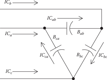
FIGURE 9.4
Delta-connected capacitor bank.

The individual phase capacitor units are specified in kvar and kV. For the delta-connected capacitors, the kV must be the line-to-line voltage. The constant susceptance for each unit can be computed in Siemens. The susceptance of a capacitor unit is computed by:

$B_{c} = \frac{k V A r}{k V_{L L}^{2} \cdot 1000} S$ (9.18)

With the susceptance computed, the delta currents serving the capacitor bank are given by:

$\begin{array}{l} I_{C}_{_{a b}} = j B_{a} \cdot V_{a b} \\ I_{C}_{_{b c}} = j B_{b} \cdot V_{b c} \\ I_{C}_{_{c a}} = j B_{c} \cdot V_{c a} \end{array}$ (9.19)

The line currents flowing into the delta-connected capacitors are computed by applying Kirchhoff’s Current Law at each node. In matrix form, the equations are:

$[\begin{matrix} I_{C}_{_{a}} \\ I_{C}_{_{b}} \\ I_{C}_{_{c}} \end{matrix}] = [\begin{matrix} 1 & 0 & - 1 \\ - 1 & 1 & 0 \\ 0 & - 1 & 1 \end{matrix}] \cdot [\begin{matrix} I_{C}_{_{a b}} \\ I_{C}_{_{b c}} \\ I_{C}_{_{c a}} \end{matrix}]$ (9.20)

9.5 Three-Phase Induction Machine

The analysis of an induction machine (motor or generator) when operating with unbalanced voltage conditions has traditionally been performed using the method of symmetrical components. In this section, the symmetrical component analysis method will be used to establish a base line for the machine operation. Once the sequence currents and voltages in the machine have been determined, they are converted to the phase domain. A direct analysis of the machine in the phase domain is introduced and is employed for the analysis of both motors and generators.

9.5.1 Induction Machine Model

The equivalent positive and negative sequence networks for an induction machine can be represented by the circuit in Figure 9.5. Because all induction machines are connected either in an ungrounded wye or in delta, there will not be any zero sequence currents and voltages; therefore, only the positive and negative sequence networks are analyzed. In the circuit in Figure 9.5, the power consumed by the resistors ( $R_{L}_{_{i}}$ ) represents the electrical power being converted to shaft power.

images

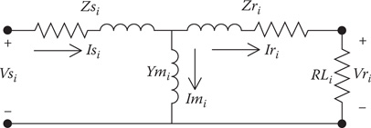
FIGURE 9.5
Sequence network.

In Figure 9.5:

i = 1 for the positive sequence circuit
i = 2 for the negative sequence circuit

The given parameters for the induction machine are assumed to be:

$\begin{array}{l} k V A_{3} = H P = three phase rating \\ k V A_{1} = \frac{k V A_{3}}{3} = single-phase rating \\ V_{L L} : rated line-to-line voltage \\ V_{L N} = \frac{V_{L L}}{\sqrt{3}} : rated line to neutral voltage \\ Z_{s} = R_{s} + j X_{s} : stator sequence impedance in per-unit \\ Z_{r} = R_{r} + j X_{r} : rotor sequence impedance in per-unit \\ Z_{m} = j X_{m} : magnetizing impedance in per-unit \end{array}$

The impedances must be converted to actual impedances in ohms. Two sets of base values are needed. The impedances in ohms are computed for the wye and delta connections by:

$\begin{array}{l} Wye Delta \\ I_{Y}_{_{base}} = \frac{k V A_{1} \cdot 1000}{V_{L N}} I_{D}_{_{base}} = \frac{k V A_{1} \cdot 1000}{V_{L L}} \\ Z_{Y}_{_{base}} = \frac{V_{L N}}{I_{Y}_{_{base}}} Z_{D}_{_{base}} = \frac{V_{L L}}{I_{D}_{_{base}}} \\ Z_{Y}_{_{Ω}} = Z_{pu} \cdot Z Y_{base} Z_{D}_{_{Ω}} = Z_{pu} \cdot Z_{D}_{_{base}} \end{array}$ (9.21)

Typically, the sequence networks are assumed to be a wye connection. When the motor is delta-connected, the computation for the impedances inside the delta is shown in Equation 9.21. These delta impedances are equal and can be converted to an equivalent wye by dividing by three. As it turns out, these values of the machine impedances in ohms will be the same as that computed using the wye-connected base values.

$Z_{Y}_{_{Ω}} = \frac{Z_{D}_{_{Ω}}}{3}$ (9.22)

Example 9.2

A three-phase induction machine is rated:

$150 kVA, 480 line-to-line volts, P_{F W} = 3.25 kW$

$Z_{s}_{_{pu}} = 0.0651 + j 0.1627, Z_{r}_{_{pu}} = 0.0553 + j 0.1139, Z_{m}_{_{pu}} = j 4.0690$

Determine the wye and delta impedances in ohms.Set base values:

$\begin{array}{l} k V A_{base} = 150 \\ k V A_{1}_{_{base}} = \frac{150}{3} = 50 \end{array}$

$\begin{array}{l} k V_{L L}_{_{base}} = \frac{480}{1000} = 0.48 \\ k V_{L N}_{_{base}} = \frac{k V_{L L}_{_{base}}}{\sqrt{3}} = 0.2771 \end{array}$

Base values for wye connection:

$\begin{array}{l} I_{Y}_{_{base}} = \frac{k V A_{1}_{_{base}}}{k V_{L N}_{_{base}}} = 180.42 \\ Z_{Y}_{_{base}} = \frac{k V_{L N}_{_{base}} \cdot 1000}{I_{Y}_{_{base}}} = 1.536 \\ Z_{Y}_{_{base}} = \frac{k V_{L N} {_{_{base}}}^{2} \cdot 1000}{k V A_{1}_{_{base}}} = \frac{{(\frac{k V_{L L}_{_{base}}}{\sqrt{3}})}^{2} \cdot 1000}{\frac{k V A_{base}}{3}} \\ Z_{Y}_{_{base}} = \frac{k V_{L L} {_{_{base}}}^{2} \cdot 1000}{k V A_{base}} = 1.536 \end{array}$

Wye-connected impedances in ohms:

$\begin{array}{l} Z_{s =} Z_{s}_{_{pu}} \cdot Z_{Y}_{_{base}} = 0.1 + j 0.2499 Ω \\ Z_{r} = Z_{r}_{_{pu}} \cdot Z_{Y}_{_{base}} = 0.0849 + j 0.175 Ω \\ Z_{m} = Z_{m}_{_{pu}} \cdot Z_{Y}_{_{base}} = j 6.2501 Ω \end{array}$

Base values for delta connection:

$\begin{array}{l} I_{D}_{_{base}} = \frac{k V A_{1}_{_{base}}}{k V_{L L}_{_{base}}} = 104.1667 \\ Z_{D}_{_{base}} = \frac{k V_{L L}_{_{base}} \cdot 1000}{I_{D}_{_{base}}} = 4.608 \\ Z_{D}_{_{base}} = \frac{k V_{L L} {_{_{base}}}^{2} \cdot 1000}{k V A_{1}_{_{base}}} = \frac{k V_{L L} {_{_{base}}}^{2} \cdot 1000}{\frac{k V A_{base}}{3}} \\ Z_{D}_{_{base}} = 3 \cdot \frac{k V_{L L} {_{_{base}}}^{2} \cdot 1000}{k V A_{base}} = 3 \cdot Z_{Y}_{_{base}} \end{array}$

Delta-connected impedances in ohms:

$\begin{array}{l} Z_{D}_{_{s}} = Z_{s}_{_{pu}} \cdot Z_{D}_{_{base}} = 0.3 + j .7497 Ω \\ Z_{D}_{_{r}} = Z_{r}_{_{pu}} \cdot Z_{D}_{_{base}} = 0.2548 + j 0.5249 Ω \\ Z_{D}_{_{m}} = Z_{m}_{_{pu}} \cdot Z_{D}_{_{base}} = 18.7504 Ω \end{array}$

Note that converting the delta impedances to wye impedances in ohms results in the same values by using the wye base values.

$\begin{array}{l} Z_{s}_{_{i}} = \frac{Z_{D}_{_{s}}}{3} = R_{s} + j X_{s} = 0.1 + j 0.2499 Ω \\ Z_{r}_{_{i}} = \frac{Z_{D}_{_{r}}}{3} = R_{r} + X_{r} = 0.0849 + j 0.175 Ω \\ Z_{m}_{_{i}} = \frac{Z_{D}_{_{m}}}{3} = j X_{m} = j 6.2501 Ω \\ Y_{m}_{_{i}} = \frac{1}{Z_{m}_{_{i}}} = - j 16 S \end{array}$

where

$\begin{array}{l} i = 1 positive sequence \\ i = 2 negative sequence \end{array}$

9.5.2 Symmetrical Component Analysis of a Motor

In Figure 9.5, the motor sequence resistances are given by:

$R_{L}_{_{i}} = \frac{1 - s_{i}}{s_{i}} \cdot R_{r}_{_{i}}$ (9.23)

where

$\begin{array}{l} positive sequence slip = s_{1} = \frac{n_{s} - n_{r}}{n_{s}} \\ negative sequence slip = s_{2} = 2 - s_{1} \\ n_{s} = synchronous speed in rpm = \frac{120 \cdot f}{p} \\ f = synchronous speed \\ p = number of poles \\ n_{r} = rotor speed in rpm \end{array}$

Note that the negative sequence load resistance will be a negative value that will lead to a negative component of shaft power.

The positive and negative sequence networks can be analyzed individually, and then sequence currents and voltages are converted to phase components. At this point, it is assumed that the stator line-to-line voltages are known. When only the magnitudes of the line-to-line voltages are known, the Law of Cosines is used to establish the angles on the voltages. The equivalent line-to-neutral voltages are needed for the analysis of the sequence networks. The line-to-neutral voltages are computed by:

$\begin{array}{l} [V_{L L}_{_{a b c}}] = [\begin{matrix} V_{a b} \\ V_{b c} \\ V_{c a} \end{matrix}] \\ [V_{L N}_{_{a b c}}] = [W] \cdot [V_{L L}_{_{a b c}}] = [\begin{matrix} V_{a n} \\ V_{b n} \\ V_{c n} \end{matrix}] \end{array}$ (9.24)

where

$[W] = \frac{1}{3} \cdot [\begin{matrix} 2 & 1 & 0 \\ 0 & 2 & 1 \\ 1 & 0 & 2 \end{matrix}]$

The computed line-to-neutral voltages are converted to sequence voltages by:

$[V_{s}_{_{012}}] = {[A]}^{- 1} \cdot [V_{L N}_{_{a b c}}] = [\begin{matrix} 0 \\ V s_{1} \\ V s_{2} \end{matrix}]$ (9.25)

where

$\begin{array}{l} [A] = [\begin{matrix} 1 & 1 & 1 \\ 1 & a^{2} & a \\ 1 & a & a^{2} \end{matrix}] \\ a = 1 \underset{____}{/ 120} \end{array}$

With the stator sequence voltages computed, the circuits of Figure 9.5 are analyzed to compute the sequence stator and rotor currents. The sequence input impedances for i = 1 and 2 are:

$Z_{in}_{_{i}} = Z_{s}_{_{i}} + \frac{Z_{m}_{_{i}} \cdot (Z_{r}_{_{i}} + R_{L}_{_{i}})}{Z_{m}_{_{i}} + Z_{r}_{_{i}} + R_{L}_{_{i}}}$ (9.26)

The stator input sequence currents are:

$\begin{array}{l} I_{s}_{_{i}} = \frac{V_{s}_{_{i}}}{Z_{in}_{_{i}}} \\ [I_{s}_{_{012}}] = [\begin{matrix} 0 \\ I_{s}_{_{1}} \\ I_{s}_{_{2}} \end{matrix}] \end{array}$ (9.27)

The rotor currents and voltages are computed by:

$\begin{array}{l} V_{m}_{_{i}} = V_{s}_{_{i}} - Z_{s}_{_{i}} \cdot I_{s}_{_{i}} \\ I_{m}_{_{i}} = \frac{V_{m}_{_{i}}}{Z_{m}_{_{i}}} \\ I_{r}_{_{i}} = I_{s}_{_{i}} - I_{m}_{_{i}} \\ V_{r}_{_{i}} = V_{m}_{_{i}} - Z_{r}_{_{i}} \cdot I_{r}_{_{i}} \\ or: V_{r}_{_{i}} = R_{L}_{_{i}} \cdot I_{r}_{_{i}} \\ [I_{r}_{_{012}}] = [\begin{matrix} 0 \\ I_{r}_{_{1}} \\ I_{r}_{_{2}} \end{matrix}] \\ [V_{r}_{_{012}}] = [\begin{matrix} 0 \\ V_{r}_{_{1}} \\ V_{r}_{_{2}} \end{matrix}] \end{array}$ (9.28)

After the sequence voltages and currents have been computed, they are converted to phase components by:

$\begin{array}{l} [I_{s}_{_{a b c}}] = [A] \cdot [I_{s}_{_{012}}] \\ [I_{r}_{_{a b c}}] = [A] \cdot [I_{r}_{_{012}}] \\ [V_{r}_{_{a b c}}] = [A] \cdot [V_{r}_{_{012}}] \end{array}$ (9.29)

The various complex powers are computed by:

$\begin{array}{l} S_{s}_{{_{a b c}}_{_{i}}} = \frac{V_{s}_{{_{a b c}}_{_{i}}} \cdot {(I_{s}_{{_{a b c}}_{_{i}}})}^{*}}{1000} \\ S_{s}_{_{total}} = \sum_{k = 1}^{3} S_{s}_{{_{a b c}}_{_{k}}} = P_{s}_{_{total}} + j Q_{s}_{_{total}} kW + j k v a r \\ S_{r}_{{_{a b c}}_{_{i}}} = \frac{V_{r}_{{_{a b c}}_{_{i}}} \cdot {(I_{r}_{{_{a b c}}_{_{i}}})}^{*}}{1000} \\ S_{r}_{_{total}} = \sum_{k = 1}^{3} S_{r}_{{_{total}}_{_{k}}} = P_{converted} kW \end{array}$ (9.30)

Example 9.3

The motor of Example 9.2 is operating with a positive sequence slip of 0.035 and line-to-line input voltages of:

$[V_{L L}_{_{a b c}}] = [\begin{matrix} 480 \underset{__}{/ 0} \\ 490 \underset{______}{/ - 121.4} \\ 475 \underset{_____}{/ 118.3} \end{matrix}]$

Compute:Stator and rotor currentsLoad output voltagesInput and output complex powersThe line-to-neutral input phase and sequence voltages are:

$\begin{array}{l} [V_{s}_{_{a b c}}] = [W] \cdot [V_{L L}_{_{a b c}}] = [\begin{matrix} 273.2 \underset{____}{/ - 30.7} \\ 281.9 \underset{____}{/ - 150.4} \\ 279.1 \underset{____}{/ 87.9} \end{matrix}] \\ [V_{s}_{_{012}}] = {[A]}^{- 1} \cdot [V_{s}_{_{a b c}}] = [\begin{matrix} 0 \\ 278.1 \underset{____}{/ - 31.0} \\ 5.1 \underset{____}{/ 130.1} \end{matrix}] \end{array}$

The positive and negative sequence stator voltages are:

$[V_{s}] = [\begin{matrix} 278.1 \underset{____}{/ - 31.0} \\ 5.1 \underset{____}{/ 130.1} \end{matrix}]$

The input stator sequence impedances are:

$\begin{array}{l} For: k = 1 and 2 \\ Z_{in}_{_{k}} = Z_{s} + \frac{Z_{m} \cdot (Z_{r} + R_{L}_{_{k}})}{Z_{m} + Z_{r} + R_{L}_{_{k}}} = [\begin{matrix} 2.1090 + j 1.1786 \\ 0.1409 + j 0.4204 \end{matrix}] \end{array}$

The positive and negative sequence stator, magnetizing, and rotor currents are:

$\begin{array}{l} I_{s}_{_{k}} = \frac{V_{s}_{_{k}}}{Z_{in}_{_{k}}} = [\begin{matrix} 115.1 \underset{______}{/ - 60.2} \\ 11.5 \underset{____}{/ 58.6} \end{matrix}] \\ V_{m}_{_{k}} = V_{s}_{_{k}} - Z_{s} \cdot I_{s}_{_{k}} = [\begin{matrix} 254.7 \underset{____}{/ - 35.4} \\ 2.0 \underset{____}{/ 135.1} \end{matrix}] \\ I_{m}_{_{k}} = \frac{V_{m}_{_{k}}}{Z_{m}} = [\begin{matrix} 40.8 \underset{____}{/ - 125.4} \\ 0.3 \underset{____}{/ 45.1} \end{matrix}] \\ I_{r}_{_{k}} = I_{s}_{_{k}} - I_{m}_{_{k}} = [\begin{matrix} 104.7 \underset{_____}{/ - 39.6} \\ 11.2 \underset{____}{/ 59.0} \end{matrix}] \end{array}$

The sequence current arrays are:

$\begin{array}{l} [I_{s}_{_{012}}] = [\begin{matrix} 0 \\ I_{s}_{_{1}} \\ I_{s}_{_{2}} \end{matrix}] = [\begin{matrix} 0 \\ \begin{matrix} 115.1 \underset{______}{/ - 60.2} \\ 11.5 \underset{____}{/ 58.6} \end{matrix} \end{matrix}] \\ [I_{r}_{_{012}}] = [\begin{matrix} 0 \\ I_{r}_{_{1}} \\ I_{r}_{_{2}} \end{matrix}] = [\begin{matrix} 0 \\ \begin{matrix} 104.7 \underset{_____}{/ - 39.6} \\ 11.2 \underset{____}{/ 59.0} \end{matrix} \end{matrix}] \end{array}$

The stator and rotor phase currents are:

$\begin{array}{l} [I_{s}_{_{a b c}}] = [A] \cdot [I_{s}_{_{012}}] = [\begin{matrix} 110.0 \underset{_____}{/ - 55.0} \\ 126.6 \underset{____}{/ 179.7} \\ 109.6 \underset{____}{/ 54.6} \end{matrix}] \\ [I_{r}_{_{a b c}}] = [A] \cdot [I_{r}_{_{012}}] = [\begin{matrix} 103.7 \underset{_____}{/ - 33.4} \\ 115.2 \underset{_____}{/ - 161.6} \\ 96.2 \underset{____}{/ 76.3} \end{matrix}] \end{array}$

The rotor sequence and phase voltages are:

$\begin{array}{l} V_{r}_{_{k}} = I_{r}_{_{k}} \cdot R_{L}_{_{k}} = [\begin{matrix} 245.2 \underset{____}{/ - 39.6} \\ 0.5 \underset{____}{/ - 121.0} \end{matrix}] \\ [V_{r}_{_{012}}] = [\begin{matrix} 0 \\ \begin{matrix} 245.2 \underset{____}{/ - 39.6} \\ 0.5 \underset{____}{/ - 121.0} \end{matrix} \end{matrix}] \\ [V_{r}_{_{a b c}}] = [A] \cdot [V_{r}_{_{012}}] = [\begin{matrix} 245.3 - 39.7____ \\ 244.7 \underset{____}{/ - 159.5} \\ 245.5 \underset{____}{/ 80.5} \end{matrix}] \end{array}$

The input and output complex powers are:

$\begin{array}{l} For i = 1, 2, 3 \\ S_{s}_{{_{a b c}}_{_{i}}} = \frac{V_{s}_{{_{a b c}}_{_{i}}} \cdot {(I_{s}_{{_{a b c}}_{_{k}}})}^{*}}{1000} = [\begin{matrix} 27.4 + j 12.4 \\ 30.9 + j 17.8 \\ 25.6 + j 16.8 \end{matrix}] \\ S_{s}_{_{total}} = \sum_{k - 1}^{3} S_{s}_{{_{a b c}}_{_{k}}} = 83.87 + j 47.00 kW + j k v a r \\ S_{r}_{{_{a b c}}_{_{i}}} = \frac{V_{r}_{{_{a b c}}_{_{i}}} \cdot {(I 4_{a b c_{k}})}^{*}}{1000} = [\begin{matrix} 25.3 + j 2.8 \\ 28.2 + j 1.0 \\ 23.6 + j 1.7 \end{matrix}] \\ S_{r}_{_{total}} = \sum_{k = 1}^{3} S_{r}_{{_{a b c}}_{_{k}}} = 77.03 kW \\ P_{loss} = Re (S_{s}_{_{total}}) - Re (S_{r}_{_{total}}) = 6.84 kW \end{array}$

9.5.3 Phase Analysis of an Induction Motor [1]

In the previous section, the analysis starts by converting known phase voltages to sequence voltages. These sequence voltages are then used to compute the stator and rotor sequence currents along with the rotor output sequence voltages. The sequence currents and voltages are then converted to phase components. In the following sections, methods will be developed where the total analysis is performed only using the phase domain.

When the positive sequence slip (s₁) is known, the input sequence impedances for the positive and negative sequence networks can be determined as:

$Z_{M}_{_{i}} = R_{s}_{_{i}} + j X_{s}_{_{i}} + \frac{(j X_{m}_{_{i}}) \cdot (R_{r}_{_{i}} + R_{L}_{_{i}} + j X_{r}_{_{i}})}{R_{r}_{_{i}} + R_{L}_{_{i}} + j (X_{m}_{_{i}} + X_{r}_{_{i}})}$ (9.31)

Once the input sequence impedances have been determined, the analysis of an induction machine operating with unbalance voltages requires the following steps:

Step 1: Transform the known line-to-line voltages to sequence line-to-line voltages.
$[\begin{matrix} V_{a b}_{_{0}} \\ V_{a b}_{_{1}} \\ V_{a b}_{_{2}} \end{matrix}] = \frac{1}{3} [\begin{matrix} 1 & 1 & 1 \\ 1 & a & a^{2} \\ 1 & a^{2} & a \end{matrix}] \cdot [\begin{matrix} V_{a b} \\ V_{b c} \\ V_{c a} \end{matrix}]$ (9.32)
In Equation 9.32, $V_{a b_{0}}$ = 0 because of Kirchhoff’s Voltage Law (KVL).
Equation 9.32 can be written as:
$[V_{L L}_{_{012}}] = {[A]}^{- 1} \cdot [V_{L L}_{_{a b c}}]$ (9.33)
Step 2: Compute the sequence line-to-neutral voltages from the line-to-line voltages:
When the machine is connected either in delta or in ungrounded wye, the zero sequence line-to-neutral voltage can be assumed to be zero. The sequence line-to-neutral voltages as a function of the sequence line-to-line voltages are given by:
$\begin{array}{l} V_{a n}_{_{0}} = V_{a b}_{_{0}} = 0 \\ V_{a n}_{_{1}} = t^{*} \cdot V_{a b}_{_{1}} \\ V_{a n}_{_{2}} = t \cdot V_{a b}_{_{2}} \end{array}$ (9.34)
where
$t = \frac{1}{\sqrt{3}} \underset{____}{/ 30}$
Equations 9.34 can be put into matrix form:
$\begin{array}{l} [\begin{matrix} V_{a n}_{_{0}} \\ V_{a n}_{_{1}} \\ V_{a n}_{_{2}} \end{matrix}] = [\begin{matrix} 1 & 0 & 0 \\ 0 & t^{*} & 0 \\ 0 & 0 & t \end{matrix}] \cdot [\begin{matrix} V_{a b}_{_{0}} \\ V_{a b}_{_{1}} \\ V_{a b}_{_{2}} \end{matrix}] \\ [V_{L N}_{_{012}}] = [T] \cdot [V_{L L}_{_{012}}] \end{array}$ (9.35)
where
$[T] = [\begin{matrix} 1 & 0 & 0 \\ 0 & t^{*} & 0 \\ 0 & 0 & t \end{matrix}]$
Step 3: Compute the sequence line currents flowing into the machine:
$\begin{array}{l} I_{a}_{_{0}} = 0 \\ I_{a}_{_{1}} = \frac{V_{a n}_{_{1}}}{Z_{M}_{_{1}}} \\ I_{a}_{_{2}} = \frac{V_{a n}_{_{2}}}{Z_{M}_{_{2}}} \end{array}$ (9.36)
Step 4: Transform the sequence currents to phase currents:
$[I_{a b c}] = [A] \cdot [I_{012}]$ (9.37)

where

$\begin{array}{l} [A] = [\begin{matrix} 1 & 1 & 1 \\ 1 & a^{2} & a \\ 1 & a & a^{2} \end{matrix}] \\ a = 1 \underset{____}{/ 120} \end{array}$

The four steps outlined previously can be performed without actually computing the sequence voltages and currents. The procedure basically reverses the steps.

Define:

$Y_{M}_{_{i}} = \frac{1}{Z_{M}_{_{i}}}$ (9.38)

The sequence currents are:

$\begin{array}{l} I_{0} = 0 \\ I_{1} = Y_{M}_{_{1}} \cdot V_{a n}_{_{1}} \\ I_{2} = Y_{M}_{_{2}} \cdot V_{a n}_{_{2}} \end{array}$ (9.39)

Since I₀ and Vab₀ are both zero, the following relationship is true:

$I_{0} = V_{a b}_{_{0}} = 0$ (9.40)

Equations 9.39 and 9.40 can be put into matrix form:

$\begin{array}{l} [\begin{matrix} I_{0} \\ I_{1} \\ I_{2} \end{matrix}] = [\begin{matrix} 1 & 0 & 0 \\ 0 & Y_{M}_{_{1}} & 0 \\ 0 & 0 & Y_{M}_{_{2}} \end{matrix}] \cdot [\begin{matrix} V_{a n}_{_{0}} \\ V_{a n}_{_{1}} \\ V_{a n}_{_{2}} \end{matrix}] \\ [I_{012}] = [Y_{M}_{_{012}}] \cdot [V_{L N}_{_{012}}] \end{array}$ (9.41)

where

$[Y_{M}_{_{012}}] = [\begin{matrix} 1 & 0 & 0 \\ 0 & Y_{M}_{_{1}} & 0 \\ 0 & 0 & Y_{M}_{_{2}} \end{matrix}]$

Substitute Equation 9.35 into Equation 9.41:

$[I_{012}] = [Y_{M}_{_{012}}] \cdot [T] \cdot [V_{L L}_{_{012}}]$ (9.42)

From symmetrical component theory:

$[V_{L L}_{_{012}}] = {[A]}^{- 1} \cdot [V_{L L}_{_{a b c}}]$ (9.43)

$[I_{a b c}] = [A] \cdot [I_{012}]$ (9.44)

Substitute Equation 9.43 into Equation 9.42, and substitute the resultant equation into Equation 9.44 to get:

$[I_{a b c}] = [A] \cdot [T] \cdot [Y_{M}_{_{012}}] \cdot {[A]}^{- 1} \cdot [V_{L L}_{_{a b c}}]$ (9.45)

Define:

$[Y_{M}_{_{a b c}}] = [A] \cdot [T] \cdot [Y_{M}_{_{012}}] \cdot {[A]}^{- 1}$ (9.46)

Therefore:

$[I_{a b c}] = [Y_{M}_{_{a b c}}] \cdot [V_{L L}_{_{a b c}}]$ (9.47)

The induction machine “phase frame admittance matrix” [YM_abc] is defined in Equation 9.46. Equation 9.47 is used to compute the input phase currents of the machine as a function of the phase line-to-line terminal voltages. This is the desired result. Recall that [YM_abc] is a function of the slip of the machine, so that a new matrix must be computed every time the slip changes.

Equation 9.47 can be used to solve for the line-to-line voltages as a function of the line currents by:

$[V_{L L}_{_{a b c}}] = [Z_{M}_{_{a b c}}] \cdot [I_{a b c}]$ (9.48)

where

$[Z_{M}_{_{a b c}}] = {[Y_{M}_{_{a b c}}]}^{- 1}$

As was done in Chapter 8, it is possible to replace the line-to-line voltages in Equation 9.48 with the “equivalent” line-to-neutral voltages:

$[V_{L N}_{_{a b c}}] = [W] \cdot [V_{L L}_{_{a b c}}]$ (9.49)

where

$[W] = [A] \cdot [T] \cdot {[A]}^{- 1} = \frac{1}{3} \cdot [\begin{matrix} 2 & 1 & 0 \\ 0 & 2 & 1 \\ 1 & 0 & 2 \end{matrix}]$

The matrix [W] is a very useful matrix that allows the determination of the “equivalent” line-to-neutral voltages from the line-to-line voltages. It is important to know that if the feeder serving the motor is grounded wye, then there will be line-to-ground voltages at the motor terminals. Because the motor is either ungrounded wye or delta, it will be necessary to convert the feeder line-to-ground voltages to line-to-line voltages and then apply Equation 9.48 to compute the equivalent line-to-neutral voltages of the motor. Equation 9.48 can be substituted into Equation 9.49 to define the “line-to-neutral” impedance equation.

$\begin{array}{l} [V_{L N}_{_{a b c}}] = [W] \cdot [Z_{M}_{_{a b c}}] \cdot [I_{a b c}] \\ [V_{L N}_{_{a b c}}] = [Z_{L N}_{_{a b c}}] \cdot [I_{a b c}] \end{array}$ (9.50)

where

$[Z_{L N}_{_{a b c}}] = [W] \cdot [Z_{M}_{_{a b c}}]$

The inverse of Equation 9.50 can be taken to determine the line currents as a function of the equivalent line-to-neutral voltages.

$[I_{a b c}] = [Y_{L N}_{_{a b c}}] \cdot [V_{L N}_{_{a b c}}]$ (9.51)

where

$[Y_{L N}_{_{a b c}}] = {[Z_{L N}_{_{a b c}}]}^{- 1}$

Care must be taken in applying Equation 9.51 to ensure that the voltages used are the equivalent line-to-neutral, not the line-to-ground, voltages. As was pointed out earlier, when the line-to-ground voltages are known, they must first be converted to the line-to-line values, and then Equation 9.49 should be used to compute the line-to-neutral voltages.

Once the machine terminal currents and line-to-neutral voltages are known, the input phase complex powers and the total three-phase input complex power can be computed.

$\begin{array}{l} S_{a} = V_{a n} \cdot {(I_{a})}^{*} \\ S_{b} = V_{b n} \cdot {(I_{b})}^{*} \\ S_{c} = V_{c n} \cdot {(I_{c})}^{*} \\ S_{Total} = S_{a} + S_{b} + S_{c} \end{array}$ (9.52)

Mostly, the only voltages known will be the magnitudes of the three line-to-line voltages at the machine terminals. When this is the case, the Law of Cosines must be used to compute the angles associated with the measured magnitudes.

Example 9.4

The induction machine in Example 9.2 is operating such that:

$\begin{array}{l} [V_{L L}_{_{a b c}}] = [\begin{matrix} V_{s}_{_{a b}} \\ V_{s}_{_{b c}} \\ V_{s}_{_{c a}} \end{matrix}] = [\begin{matrix} 480.0 \underset{____}{/ 0} \\ 490 \underset{____}{/ - 121.4} \\ 475 \underset{____}{/ 118.3} \end{matrix}] V \\ Positive sequence slip: s_{1} = 0.035 \end{array}$

Determine the input line currents and complex power input to the machine (motor).Compute the negative sequence slip:

$s_{2} = 2 - s_{1} = 1.965$

Compute the sequence load resistance values:

$R_{L}_{_{i}} = \frac{1 - s_{i}}{s_{i}} \cdot R_{r}_{_{i}} = [\begin{matrix} 2.3408 \\ - 0.0417 \end{matrix}]$

Calculate the input sequence impedances and admittances:

$\begin{array}{l} Z_{M}_{_{i}} = Z_{s}_{_{i}} + \frac{Z_{m}_{_{i}} \cdot (Z_{r}_{_{i}} + R_{L}_{_{i}})}{Z_{m}_{_{i}} + Z_{r}_{_{i}} + R_{L}_{_{i}}} = [\begin{matrix} 2.109 + j 1.1786 \\ 0.1409 + j 0.4204 \end{matrix}] \\ Y_{M}_{_{i}} = \frac{1}{Z_{M}_{_{i}}} = [\begin{matrix} 0.3613 - j 0.2019 \\ 0.7166 - j 2.1385 \end{matrix}] \end{array}$

Define the T, A, and W matrices:

$\begin{array}{l} t = \frac{1}{\sqrt{3}} \cdot \underset{____}{/ 30} [T] = [\begin{matrix} 1 & 0 & 0 \\ 0 & t^{*} & 0 \\ 0 & 0 & t \end{matrix}] \\ a = 1 \underset{____}{/ 120} [A] = [\begin{matrix} 1 & 1 & 1 \\ 1 & a^{2} & a \\ 1 & a & a^{2} \end{matrix}] \\ [W] = \frac{1}{3} \cdot [\begin{matrix} 2 & 1 & 0 \\ 0 & 2 & 1 \\ 1 & 0 & 2 \end{matrix}] \end{array}$

Define the sequence input admittance matrix:

$[Y_{M}_{_{012}}] = [\begin{matrix} 1 & 0 & 0 \\ 0 & Y_{M}_{_{1}} & 0 \\ 0 & 0 & Y_{M}_{_{2}} \end{matrix}] = [\begin{matrix} 1 & 0 & 0 \\ 0 & 0.3613 - j 0.2019 & 0 \\ 0 & 0 & 0.7166 - j 2.1385 \end{matrix}]$

Compute the phase input admittance matrix:

$[Y_{M}_{_{a b c}}] = [A] \cdot [T] \cdot [Y_{M}_{_{012}}] \cdot {[A]}^{- 1} = [\begin{matrix} 0.6993 - j 0.3559 & - 0.0394 - j 0.0684 & 0.34 + j 0.4243 \\ 0.34 + j 0.4243 & 0.6993 - j 0.3559 & - 0.0394 - j 0.0684 \\ - 0.0394 - j 0.0684 & 0.34 + j 0.4243 & 0.6993 - j 0.3559 \end{matrix}]$

Compute input line currents:

$[I_{s}_{_{a b c}}] = [Y_{M}_{_{a b c}}] \cdot [V_{L L}_{_{a b c}}] = [\begin{matrix} 110.0 \underset{____}{/ - 55.0} \\ 126.6 \underset{____}{/ 179.7} \\ 109.6 \underset{____}{/ 54.6} \end{matrix}]$

Compute line-to-neutral voltages:

$[V_{L N}_{_{a b c}}] = [W] \cdot [V_{L L}_{_{a b c}}] = [\begin{matrix} 273.2 \underset{______}{/ - 30.7} \\ 281.9 \underset{____}{- 150.4} \\ 279.1 \underset{____}{/ 87.9} \end{matrix}]$

Compute the stator complex input power:

$\begin{array}{l} For j = 1, 2, 3 \\ S_{s}_{_{j}} = \frac{V_{L N}_{{_{a b c}}_{_{j}}} \cdot {(I_{s}_{{_{a b c}}_{_{j}}})}^{*}}{1000} = [\begin{matrix} 27.4 + j 12.4 \\ 30.9 + j 17.8 \\ 25.6 + j 16.8 \end{matrix}] \\ S_{s}_{_{total}} = 83.9 + j 47.0 kW + j k v a r \end{array}$

Note that these are the same results as in Example 9.3, and only fewer steps are required.

9.5.4 Voltage and Current Unbalance [2]

Three-phase distribution feeders are unbalanced because of conductor spacings and the unbalanced loads served. Because of this, the line-to-line voltages serving an induction motor will be unbalanced. When a motor operates with unbalanced voltages, it will overheat and draw unbalanced currents that may exceed the rated current of the motor. It has become a rule of thumb to not let the voltage unbalance exceed 3%. A common way of determining voltage and current unbalance is based upon the magnitudes of the line-to-line voltages and line currents. The computation of unbalance involves three steps:

Step 1: Compute the average of the line-to-line voltages
Step 2: Compute the magnitudes of the deviation (dev) between the phase magnitudes and the average
Step 3: Compute unbalance

$Unbalance = \frac{\max (dev)}{average} \cdot 100 %$

The same three steps are used to compute current unbalance.

Example 9.5

Determine the voltage and current unbalances for the motor in Examples 9.2 and 9.3.The terminal line-to-line voltages were:

$[V_{L L}_{_{a b c}}] = [\begin{matrix} 480 \underset{____}{/ 0} \\ 490 \underset{____}{/ - 121.4} \\ 475 \underset{____}{/ 118.3} \end{matrix}]$

Step 1:

$V_{average} = \frac{1}{3} \cdot \sum_{k = 1}^{3} | V_{L L}_{{_{a b c}}_{_{k}}} | = 481.7$
Step 2:

${dev}_{i} = | | V_{L L}_{_{i}} | - V_{average} | = [\begin{matrix} 1.67 \\ 8.33 \\ 6.67 \end{matrix}]$
Step 3:

$V_{unbalance} = \frac{\max (dev)}{V_{average}} = \frac{8.33}{481.7} \cdot 100 = 1.73 %$

The line currents were:

$[I_{s}_{_{a b c}}] = [\begin{matrix} 110.0 \underset{____}{/ - 55.0} \\ 126.6 \underset{____}{/ 179.7} \\ 109.8 \underset{____}{/ 54.6} \end{matrix}]$

Step 1:

$I_{average} = \frac{1}{3} \cdot \sum_{k = 1}^{3} | I_{s}_{{_{a b c}}_{_{k}}} | = 115.4$
Step 2:

${dev}_{i} = | | I_{s}_{{_{a b c}}_{_{i}}} | - I_{average} | = [\begin{matrix} 5.39 \\ 11.20 \\ 5.82 \end{matrix}]$
Step 3:

$I_{unbalance} = \frac{\max (dev)}{I_{average}} = \frac{11.20}{115.4} \cdot 100 = 9.71 %$

9.5.5 Motor Starting Current

An induction motor under line starting will cause a current to flow that is much greater than rated. Typically, the motor is not line-started, but the input voltages will be reduced under starting conditions. The starting current can be computed by setting the positive sequence slip to 1. For the motor in Example 9.2 with the same line-to-line voltages applied, the starting currents are:

$[I_{s}_{_{a b c}}] = [\begin{matrix} 596.4 \underset{____}{/ - 97.5} \\ 615.3 \underset{____}{/ 142.8} \\ 609.2 \underset{____}{/ 21.1} \end{matrix}]$

When the starting voltage is reduced to one-half, the starting currents are:

$[I_{s}_{_{a b c}}] = [\begin{matrix} 298.2 \underset{____}{/ - 97.5} \\ 307.7 \underset{____}{/ 142.8} \\ 304.6 \underset{____}{/ 21.1} \end{matrix}]$

Note that the rated current for the motor is 180 A.

9.5.6 The Equivalent T Circuit

Once the terminal line-to-neutral voltages and currents are known, it is desired to analyze as to what happens inside the machine. In particular, the stator and rotor losses are needed in addition to the “converted” shaft power. A method of performing the internal analysis can be developed in the phase frame by starting with the equivalent T sequence networks as shown in Figure 9.6.

images

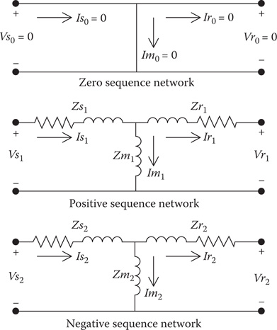
FIGURE 9.6
Induction machine equivalent T sequence networks.

The three sequence networks in Figure 9.6 can be reduced to the equivalent T sequence circuit shown in Figure 9.7.

images

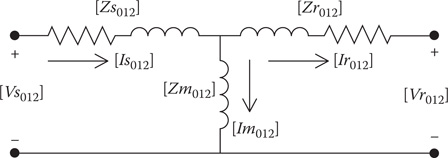
FIGURE 9.7
Sequence equivalent T circuit.

Because the zero sequence voltages and currents are always zero in Figure 9.7, the sequence matrices are defined as:

$Voltages: [V_{s}_{_{012}}] = [\begin{matrix} 0 \\ V_{s}_{_{1}} \\ V_{s}_{_{2}} \end{matrix}] [V_{r}_{_{012}}] = [\begin{matrix} 0 \\ V_{r}_{_{1}} \\ V_{r}_{_{2}} \end{matrix}]$

$Currents: [I_{s}_{_{012}}] = [\begin{matrix} 0 \\ I_{s}_{_{1}} \\ I_{s}_{_{2}} \end{matrix}] [I_{m}_{_{012}}] = [\begin{matrix} 0 \\ I_{m}_{_{1}} \\ I_{m}_{_{2}} \end{matrix}] [I_{r}_{_{012}}] = [\begin{matrix} 0 \\ I_{r}_{_{1}} \\ I_{r}_{_{2}} \end{matrix}] Impedances : [Z_{s}_{_{012}}] = [\begin{matrix} 0 & 0 & 0 \\ 0 & Z_{s}_{_{1}} & 0 \\ 0 & 0 & Z_{s}_{_{2}} \end{matrix}] [Z_{r}_{_{012}}] = [\begin{matrix} 0 & 0 & 0 \\ 0 & Z_{r}_{_{1}} & 0 \\ 0 & 0 & Z_{r}_{_{2}} \end{matrix}] [Z_{m}_{_{012}}] = [\begin{matrix} 0 & 0 & 0 \\ 0 & Z_{m}_{_{1}} & 0 \\ 0 & 0 & Z_{m}_{_{2}} \end{matrix}]$ (9.53)

The sequence voltage drops in the rotor circuit of Figure 9.7 are:

$[v_{r}_{_{012}}] = [Z_{r}_{_{012}}] \cdot [I_{r}_{_{012}}]$ (9.54)

As an example, the rotor phase voltage drops are given by:

$\begin{array}{l} [v_{r}_{_{012}}] = [Z_{r}_{_{012}}] \cdot [I_{r}_{_{012}}] \\ [v_{r}_{_{a b c}}] = [A] \cdot [V_{r}_{_{012}}] \\ [I_{r}_{_{012}}] = [A^{- 1}] \cdot [I_{r}_{_{a b c}}] \\ [v_{r}_{_{a b c}}] = [A] \cdot [Z_{r}_{_{012}}] \cdot {[A]}^{- 1} \cdot [I_{r}_{_{a b c}}] \\ [v_{r}_{_{a b c}}] = [Z_{r}_{_{a b c}}] \cdot [I_{r}_{_{a b c}}] \end{array}$ (9.55)

where

$[Z_{r}_{_{a b c}}] = [A] \cdot [Z_{r}_{_{012}}] \cdot {[A]}^{- 1}$

The same process is used on the other voltage drops, so that the circuit of Figure 9.7 can be converted to an equivalent T circuit in terms of the phase components (Figure 9.8).

images

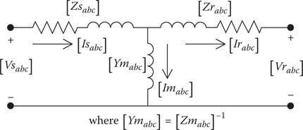
FIGURE 9.8
Phase equivalent T circuit.

The stator voltages and currents of the phase equivalent T circuit as a function of the rotor voltages and currents are defined by:

$[\begin{matrix} [V_{s}_{_{a b c}}] \\ [I_{s}_{_{a b c}}] \end{matrix}] = [\begin{matrix} [A_{m}_{_{a b c}}] & [B_{m}_{_{a b c}}] \\ [C_{m}_{_{a b c}}] & [D_{m}_{_{a b c}}] \end{matrix}] \cdot [\begin{matrix} [V_{r}_{_{a b c}}] \\ [I_{r}_{_{a b c}}] \end{matrix}]$ (9.56)

where

$\begin{array}{l} [A_{m}_{_{a b c}}] = [U] + [Z_{s}_{_{a b c}}] \cdot [Y_{m}_{_{a b c}}] \\ [B_{m}_{_{a b c}}] = [Z_{s}_{_{a b c}}] + [Z_{r}_{_{a b c}}] + [Z_{s}_{_{a b c}}] \cdot [Y_{m}_{_{a b c}}] \cdot [Z_{r}_{_{a b c}}] \\ [C_{m}_{_{a b c}}] = [Y_{m}_{_{a b c}}] \\ [D_{m}_{_{a b c}}] = [U] + [Y_{m}_{_{a b c}}] \cdot [Z_{r}_{_{a b c}}] \\ [U] = [\begin{matrix} 1 & 0 & 0 \\ 0 & 1 & 0 \\ 0 & 0 & 1 \end{matrix}] \end{array}$

The inverse of the ABCD matrices of Equation 9.56 is used to define the rotor voltages and currents as a function of the stator voltages and currents.

$\begin{array}{l} [\begin{matrix} [V_{r}_{_{a b c}}] \\ [I_{r}_{_{a b c}}] \end{matrix}] = {[\begin{matrix} [A_{m}_{_{a b c}}] & [B_{m}_{_{a b c}}] \\ [C_{m}_{_{a b c}}] & [D_{m}_{_{a b c}}] \end{matrix}]}^{- 1} \cdot [\begin{matrix} [V_{s}_{_{a b c}}] \\ [I_{s}_{_{a b c}}] \end{matrix}] \\ [\begin{matrix} V_{r}_{_{a b c}} \\ I_{r}_{_{a b c}} \end{matrix}] = [\begin{matrix} [D_{m}_{_{a b c}}] & - [B_{m}_{_{a b c}}] \\ - [C_{m}_{_{a b c}}] & [A_{m}_{_{a b c}}] \end{matrix}] \cdot [\begin{matrix} [V_{s}_{_{a b c}}] \\ [I_{s}_{_{a b c}}] \end{matrix}] \\ because [A_{m}_{_{a b c}}] \cdot [D_{m}_{_{a b c}}] - [B_{m}_{_{a b c}}] \cdot [C_{m}_{_{a b c}}] = [U] \end{array}$ (9.57)

The power converted to the shaft is given by:

$\begin{array}{l} P_{conv} = V_{r}_{_{a}} \cdot {(I_{r}_{_{a}})}^{*} + V_{r}_{_{b}} \cdot {(I_{r}_{_{b}})}^{*} + V_{r}_{_{c}} \cdot {(I_{r}_{_{c}})}^{*} \\ or: P_{conv} = \sum_{k = 1}^{3} V_{r}_{{_{a b c}}_{_{k}}} \cdot {(I_{r}_{{_{a b c}}_{_{k}}})}^{*} \end{array}$ (9.58)

The useful shaft power can be determined as a function of the rotational (FW) losses:

$P_{shaft} = P_{conv} - P_{F W}$ (9.59)

The stator total power loss is:

$\begin{array}{l} [V_{drop}_{_{s}}] = [Z_{s}_{_{a b c}}] \cdot [I_{s}_{_{a b c}}] \\ P_{stator} = Re \sum_{k = 1}^{3} (\frac{V_{drop}_{{_{s}}_{_{k}}} \cdot {(I_{s}_{{_{a b c}}_{_{k}}})}^{*}}{1000}) \end{array}$ (9.60)

The rotor total power loss is:

$\begin{array}{l} [V_{drop}_{_{r}}] = [Z_{r}_{_{a b c}}] \cdot [I_{r}_{_{a b c}}] \\ P_{rotor} = Re \sum_{k = 1}^{3} (\frac{V_{drop}_{{_{r}}_{_{k}}} \cdot {(I_{r}_{{_{a b c}}_{_{k}}})}^{*}}{1000}) \end{array}$ (9.61)

The total input complex power is:

$S_{in} = \sum_{k = 1}^{3} (\frac{V_{s}_{{_{a b c}}_{_{k}}} \cdot {(I_{s}_{{_{a b c}}_{_{k}}})}^{*}}{1000}) = P_{in} + j Q_{in} kW + j k v a r$ (9.62)

Example 9.6

For the motor in Example 9.2, determine:

ABCD matrices for the phase equivalent T circuit
Rotor output voltages and currents
Rotor converted and shaft powers
Rotor and stator “copper” losses
Total complex power input to the stator

Define the sequence impedance matrices:

$\begin{array}{l} For: Y_{m}_{_{i}} = \frac{1}{Z_{m}_{_{i}}} = - j 0.16 \\ [Z_{s}_{_{012}}] = [\begin{matrix} 0 & 0 & 0 \\ 0 & Z_{s}_{_{1}} & 0 \\ 0 & 0 & Z_{s}_{_{2}} \end{matrix}] = [\begin{matrix} 0 & 0 & 0 \\ 0 & 0.1 + j 0.2499 & 0 \\ 0 & 0 & 0.1 + j 0.2499 \end{matrix}] \\ [Z_{r}_{_{012}}] = [\begin{matrix} 0 & 0 & 0 \\ 0 & Z_{r}_{_{1}} & 0 \\ 0 & 0 & Z_{r}_{_{2}} \end{matrix}] = [\begin{matrix} 0 & 0 & 0 \\ 0 & 0.0849 + j 0.175 & 0 \\ 0 & 0 & 0.0849 + j 0.175 \end{matrix}] \\ [Y_{m}_{_{012}}] = [\begin{matrix} 0 & 0 & 0 \\ 0 & Y_{m}_{_{1}} & 0 \\ 0 & 0 & Y_{m}_{_{2}} \end{matrix}] = [\begin{matrix} 0 & 0 & 0 \\ 0 & - j 0.16 & 0 \\ 0 & 0 & - j 0.16 \end{matrix}] \end{array}$

Compute the phase impedance and admittance matrices:

$\begin{array}{l} [Z_{s}_{_{a b c}}] = [A] \cdot [Z_{s}_{_{012}}] \cdot {[A]}^{- 1} = [\begin{matrix} 0.0667 + j 0.1666 & - 0.0333 - j 0.0833 & - 0.0333 - j 0.0833 \\ - 0.0333 - j 0.0833 & 0.0667 + j 0.1666 & - 0.0333 - j 0.0833 \\ - 0.0333 - j 0.0833 & - 0.0333 - j 0.0833 & 0.0667 + j 0.1666 \end{matrix}] \\ [Z_{r}_{_{a b c}}] = [A] \cdot [Z_{r}_{_{012}}] \cdot {[A]}^{- 1} = [\begin{matrix} 0.0566 + j 0.1167 & - 0.0283 - j 0.0583 & - 0.0283 - j 0.0583 \\ - 0.0283 - j 0.0583 & 0.0566 + j 0.1167 & - 0.0283 - j 0.0583 \\ - 0.0283 - j 0.0583 & - 0.0283 - j 0.0583 & 0.0566 + j 0.1167 \end{matrix}] \\ [Y_{m}_{_{a b c}}] = [A] \cdot [Y_{m}_{_{012}}] \cdot {[A]}^{- 1} = [\begin{matrix} - j 0.1067 & j 0.0533 & j 0.0533 \\ j 0.0533 & - j 0.1067 & j 0.0533 \\ j 0.0533 & j 0.0533 & - j 0.1067 \end{matrix}] \end{array}$

Compute the phase ABCD matrices:

$\begin{array}{l} [A_{m}_{_{a b c}}] = [U] + [Z_{s}_{_{a b c}}] \cdot [Y_{m}_{_{a b c}}] = [\begin{matrix} 1.0267 - j 0.0107 & - 0.0133 + j 0.0053 & - 0.0133 + j 0.0053 \\ - 0.0133 + j 0.0053 & 1.0267 - j 0.0107 & - 0.0133 + j 0.0053 \\ - 0.0133 + j 0.0053 & - 0.0133 + j 0.0053 & 1.0267 - j 0.0107 \end{matrix}] \\ [B_{m}_{_{a b c}}] = [Z_{s}_{_{a b c}}] + [Z_{r}_{_{a b c}}] + [Z_{s}_{_{a b c}}] \cdot [Y_{m}_{_{a b c}}] \cdot [Z_{r}_{_{a b c}}] \\ [B_{m}_{_{a b c}}] = [\begin{matrix} 0.1274 + j 0.2870 & - 0.0637 - j 0.1435 & - 0.0637 - j 0.1435 \\ - 0.0637 - j 0.1435 & 0.1274 + j 0.2870 & - 0.0637 - j 0.1435 \\ - 0.0637 - j 0.1435 & - 0.0637 - j 0.1435 & 0.1274 + j 0.2870 \end{matrix}] \\ [C_{m}_{_{a b c}}] = [Y_{m}_{_{a b c}}] = [\begin{matrix} - j 0.1067 & j 0.0533 & j 0.0533 \\ j 0.0533 & - j 0.1067 & j 0.0533 \\ j 0.0533 & j 0.0533 & - j 0.1067 \end{matrix}] \\ [D_{m}_{_{A B C}}] = [U] + [Y_{m}_{_{a b c}}] \cdot [Z_{r}_{_{a b c}}] \\ [D_{m}_{_{a b c}}] = [\begin{matrix} 1.0187 - j 0.0091 & - 0.0093 + j 0.0045 & - 0.0093 + j 0.0045 \\ - 0.0093 + j 0.0045 & 1.0187 - j 0.0091 & - 0.0093 + j 0.0045 \\ - 0.0093 + j 0.0045 & - 0.0093 + j 0.0045 & 1.0187 - j 0.0091 \end{matrix}] \end{array}$

Compute the rotor output voltages and currents:

$\begin{array}{l} [V_{r}_{_{a b c}}] = [D_{m}_{_{a b c}}] \cdot [V_{s}_{_{a b c}}] - [B_{m}_{_{a b c}}] \cdot [I_{s}_{_{a b c}}] = [\begin{matrix} 245.3 \underset{____}{/ - 39.7} \\ 244.7 \underset{____}{/ - 159.5} \\ 245.6 \underset{____}{/ 80.5} \end{matrix}] \\ [I_{r}_{_{a b c}}] = - [C_{m}_{_{a b c}}] \cdot [V_{s}_{_{a b c}}] + [A_{m}_{_{a b c}}] \cdot [I_{s}_{_{a b c}}] = [\begin{matrix} 103.7 - 33.4____ \\ 115.2 \underset{____}{/ - 161.6} \\ 96.2 \underset{____}{/ 76.3} \end{matrix}] \end{array}$

Compute the rotor converted and shaft powers:

$\begin{array}{l} P_{conv} = \sum_{k = 1}^{3} \frac{V_{r}_{{_{a b c}}_{_{k}}} \cdot {(I_{r}_{{_{a b c}}_{_{k}}})}^{*}}{1000} = 77.03 kW \\ P_{shaft} = P_{conv} - P_{F W} = 77.03 - 3.25 = 73.78 kW \\ P_{H P} = \frac{73.78}{0.746} = 98.90 HP \end{array}$

Compute stator and rotor power losses:

$\begin{array}{l} [V_{drop}_{_{s}}] = [Z_{s}_{_{a b c}}] \cdot [I_{s}_{_{a b c}}] = [\begin{matrix} 29.6 \underset{____}{/ 13.2} \\ 34.1 \underset{____}{/ - 112.1} \\ 29.5 \underset{____}{/ 122.8} \end{matrix}] \\ P_{s} =Re \sum_{k = 1}^{3} \frac{V_{drop}_{{_{s}}_{_{k}}} \cdot {(I_{s}_{{_{a b c}}_{_{k}}})}^{*}}{1000} = 4.01 kW \\ [V_{drop}_{_{r}}] = [Z_{r}_{_{a b c}}] \cdot [I_{r}_{_{a b c}}] = [\begin{matrix} 20.2 \underset{____}{/ 30.7} \\ 22.4 \underset{____}{/ - 97.5} \\ 18.7 \underset{____}{/ 140.4} \end{matrix}] \\ P_{r} =Re \sum_{k = 1}^{3} \frac{V_{drop}_{{_{r}}_{_{k}}} \cdot {(I_{r}_{{_{a b c}}_{_{k}}})}^{*}}{1000} = 2.83 kW \end{array}$

Compute complex power into stator:

$\begin{array}{l} S_{in} = \sum_{k = 1}^{3} \frac{V_{s}_{{_{a b c}}_{_{k}}} \cdot {(I_{s}_{{_{a b c}}_{_{k}}})}^{*}}{1000} = 83.87 + j 47.00 \\ P_{conv} = P_{in} - P_{s} - P_{r} = 83.87 - 4.01 - 2.83 = 77.03 \end{array}$

9.5.7 Computation of Slip

When the input power to the motor is specified instead of the slip, an iterative process is required to compute the value of slip that will force the input power to be within some small tolerance of the specified input power.

The iterative process for computing the slip that will produce the specified input power starts with assuming an initial value of the positive sequence slip and a change in slip. To compute the slip the initial values are:

$\begin{array}{l} s_{old} = 0.0 \\ d s = 0.01 \end{array}$ (9.63)

The value of slip used in the first iteration is then:

$\begin{array}{l} s_{1} = s_{old} + d s \\ where s_{1} = positive sequence slip \end{array}$ (9.64)

where s1 = positive sequence slip.

With the new value of slip, the input shunt admittance matrix [YM_abc] is computed. The given line-to-line voltages are used to compute the stator currents. The [W] matrix is used to compute the equivalent line-to-neutral voltages. The total three-phase input complex power is then computed. The computed three-phase input power is compared to the specified three-phase input power. The error is computed as:

$Error = P_{specified} - P_{computed}$ (9.65)

If the error is positive, the slip needs to be increased so that the computed power will increase. This is done by:

$\begin{array}{l} s_{old} = value of slip used in previous iteration \\ s_{new} = s_{i} = s_{old} + d s \end{array}$ (9.66)

The new value of s₁ is used to repeat the calculations for the input power to the motor.

If the error is negative, it means that a bracket has been established. The required value of slip lies between s_old and s_new. In order to zero in on the required slip, the old value of slip will be used, and the change in slip will be reduced by a factor of 10.

$\begin{array}{l} d s = \frac{d s}{10} \\ s_{i} = s_{old} + d s \end{array}$ (9.67)

This process is illustrated in Figure 9.9.

images

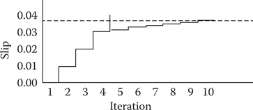
FIGURE 9.9
Slip vs. iteration.

When the slip has produced the specified input power within a specified tolerance, the T circuit is used to compute the voltages and currents in the rotor.

Example 9.7

For the induction motor and voltages in Example 9.2, determine the value of positive sequence slip that will develop 100 kW input power to the motor.To start set:

$\begin{array}{l} s_{old} = 0 \\ d s = 0.01 \\ tol = 0.01 \\ P_{computed} = 100 \end{array}$

Figure 9.10 shows a Mathcad program that computes the required slip.

images

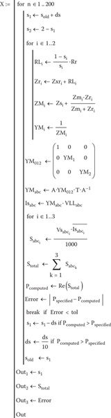
FIGURE 9.10
Mathcad program for computed required slip.

After 22 iterations, the Mathcad program gives the following results.

$\begin{array}{l} s_{1} = 0.0426 \\ S_{total} = 100.00 + j 52.54 \\ Error = 0.004 \end{array}$

Note that the motor is being supplied reactive power.

9.5.8 Induction Generator

Three-phase induction generators are becoming common as a source of distributed generation on a distribution system. In particular, Windmills generally drive an induction motor. It is, therefore, important that a simple model of an induction generator be developed for power-flow purposes. In reality, the same model as that which was used for the induction motor is used for the induction generator. The only change is that the generator will be driven at a speed in excess of synchronous speed, which means that the slip will be a negative value. The generator can be modeled with the equivalent admittance matrix from Equation 9.46.

Example 9.8

Using the same induction machine and line-to-line voltages in Examples 9.2 and 9.4, determine the slip of the machine so that it will generate 100 kW. Because the same model is being used with the same assumed direction of currents, the specified power at the terminals of the machine will be:

$P_{gen} = - 100$

As before, the initial “old” value of slip is set to 0.0. However, because the machine is now a generator, the initial change in slip will be:

$d s = - 0.01$

As before, the value of slip to be used for the first iteration will be:

$s_{1} = s_{old} + d s = - 0.01$

The same Mathcad program as that which was used in Example 9.7 is used with the exception that the two “if” statements are reversed in order to determine the new value of slip. The two equations changed are:

$\begin{array}{l} s_{i} \leftarrow s_{i} - d s if P_{computed} < P_{specified} \\ d s \leftarrow \frac{d s}{10} if P_{computed} < P_{specified} \end{array}$

After 34 iterations, the results are:

$\begin{array}{l} s_{1} = - 0.03997 \\ S_{computed} = - 99.99 + j 59.73 kW + j k v a r \\ Error = 0.0084 \end{array}$

It must be noted that even though the machine is supplying power to the system, it is still consuming reactive power. The point being that even though the induction generator can supply real power to the system, it will still require reactive power from the system. This reactive power is typically supplied by shunt capacitors or a static kvar supply at the location of the Windmill.

9.5.9 Induction Machine Thevenin Equivalent Circuit

When an induction motor is operating under load and a short circuit occurs on the feeder for a brief period of time, the motor will supply short-circuit current as a result of the stored energy in the rotating mass of the motor and load. The induction machine T circuit is modified to indicate that there is a voltage at the rotor terminals as shown in Figure 9.11.

images

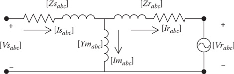
FIGURE 9.11
Induction motor phase equivalent T circuit.

The stator input line-to-neutral voltages and currents are given by:

$\begin{array}{l} [V_{s}_{_{a b c}}] = [A_{m}_{_{a b c}}] \cdot [V_{r}_{_{a b c}}] + [B_{m}_{_{a b c}}] \cdot [I_{r}_{_{a b c}}] \\ [I_{s}_{_{a b c}}] = [C_{m}_{_{a b c}}] \cdot [V_{r}_{_{a b c}}] + [D_{m}_{_{a b c}}] \cdot [I_{r}_{_{a b c}}] \end{array}$ (9.68)

Solve for the rotor current in Equation 9.68:

$[I_{r}_{_{a b c}}] = - {[D_{m}_{_{a b c}}]}^{- 1} \cdot [C_{m}_{_{a b c}}] \cdot [V_{r}_{_{a b c}}] + {[D_{m}_{_{a b c}}]}^{- 1} \cdot [I_{s}_{_{a b c}}]$ (9.69)

Substitute Equation 9.69 into Equation 9.68:

$\begin{array}{l} [V_{s}_{_{a b c}}] = [A_{m}_{_{a b c}}] \cdot [V_{r}_{_{a b c}}] + [B_{m}_{_{a b c}}] \cdot (- {[D_{m}_{_{a b c}}]}^{- 1} \cdot [C_{m}_{_{a b c}}] \cdot [V_{r}_{_{a b c}}] + {[D_{m}_{_{a b c}}]}^{- 1} \cdot [I_{s}_{_{a b c}}]) \\ [V_{s}_{_{a b c}}] = ([A_{m}_{_{a b c}}] - [B_{m}_{_{a b c}}] \cdot {[D_{m}_{_{a b c}}]}^{- 1} \cdot [C_{m}_{_{a b c}}]) \cdot [V_{r}_{_{a b c}}] + [B_{m}_{_{a b c}}] \cdot {[D_{m}_{_{a b c}}]}^{- 1} \cdot [I_{s}_{_{a b c}}] \\ Define: [E_{t h}_{_{a b c}}] = ([A_{m}_{_{a b c}}] - [B_{m}_{_{a b c}}] \cdot {[D_{m}_{_{a b c}}]}^{- 1} \cdot [C_{m}_{_{a b c}}]) \cdot [V_{r}_{_{a b c}}] \\ [Z_{t h}_{_{a b c}}] = [B_{m}_{_{a b c}}] \cdot {[D_{m}_{_{a b c}}]}^{- 1} \\ Therefore: [V_{s}_{_{a b c}}] = [E_{t h}_{_{a b c}}] + [Z_{t h}_{_{a b c}}] \cdot [I_{s}_{_{a b c}}] \end{array}$ (9.70)

The final form of Equation 9.70 reduces the T circuit to the Thevenin equivalent circuit of Figure 9.12.

images

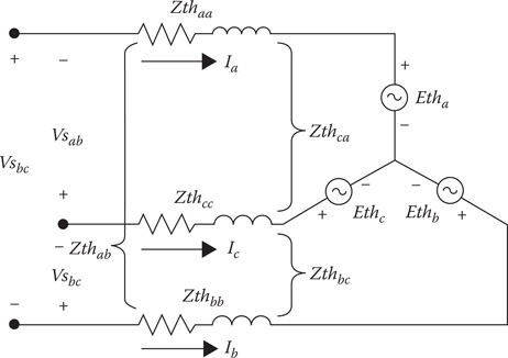
Figure 9.12
Motor Thevenin equivalent circuit.

In Figure 9.12, the Thevenin voltage drops are:

$\begin{array}{l} [\begin{matrix} v_{a} \\ v_{b} \\ v_{c} \end{matrix}] = [\begin{matrix} Z_{t h}_{_{a a}} & Z_{t h}_{_{a b}} & Z_{t h}_{_{a c}} \\ Z_{t h}_{_{b a}} & Z_{t h}_{_{b b}} & Z_{t h}_{_{b c}} \\ Z_{t h}_{_{c a}} & Z_{t h}_{_{c b}} & Z_{t h}_{_{c a}} \end{matrix}] \cdot [\begin{matrix} I_{a} \\ I_{b} \\ I_{c} \end{matrix}] \\ [v_{a b c}] = [Z_{t h}_{_{a b c}}] \cdot [I_{a b c}] \end{array}$ (9.71)

The motor terminal Thevenin line-to-line voltages are:

$\begin{array}{l} [\begin{matrix} V_{s}_{_{a b}} \\ V_{s}_{_{b c}} \\ V_{s}_{_{c a}} \end{matrix}] = [\begin{matrix} E_{t h}_{_{a}} - E_{t h}_{_{b}} \\ E_{t h}_{_{b}} - E_{t h}_{_{c}} \\ E_{t h}_{_{c}} - E_{t h}_{_{a}} \end{matrix}] + [\begin{matrix} v_{a} - v_{b} \\ v_{b} - v_{c} \\ v_{c} - v_{a} \end{matrix}] \\ Note that: [\begin{matrix} 1 & - 1 & 0 \\ 0 & 1 & - 1 \\ - 1 & 0 & 1 \end{matrix}] \cdot [\begin{matrix} v_{a} \\ v_{b} \\ v_{c} \end{matrix}] = [\begin{matrix} v_{a} - v_{b} \\ v_{b} - v_{c} \\ v_{c} - v_{a} \end{matrix}] \\ Apply the matrix [D v] \\ [\begin{matrix} V_{s}_{_{a b}} \\ V_{s}_{_{b c}} \\ V_{s}_{_{c a}} \end{matrix}] = [\begin{matrix} 1 & - 1 & 0 \\ 0 & 1 & - 1 \\ - 1 & 0 & 1 \end{matrix}] \cdot [\begin{matrix} E_{t h}_{_{a}} \\ E_{t h}_{_{b}} \\ E_{t h}_{_{c}} \end{matrix}] + [\begin{matrix} 1 & - 1 & 0 \\ 0 & 1 & - 1 \\ - 1 & 0 & 1 \end{matrix}] \cdot [\begin{matrix} v_{a} \\ v_{b} \\ v_{c} \end{matrix}] \\ [V_{s} {_{_{L L}}}_{_{_{a b c}}}] = [D v] \cdot [E_{t h}_{_{a b c}}] + [D v] \cdot [v_{a b c}] \end{array}$ (9.72)

Substitute Equation 6.71 into Equation 9.72:

$\begin{array}{l} [\begin{matrix} V_{s}_{_{a b}} \\ V_{s}_{_{b c}} \\ V_{s}_{_{c a}} \end{matrix}] = [\begin{matrix} 1 & - 1 & 0 \\ 0 & 1 & - 1 \\ - 1 & 0 & 1 \end{matrix}] \cdot [\begin{matrix} E_{t h}_{_{a}} \\ E_{t h}_{_{b}} \\ E_{t h}_{_{c}} \end{matrix}] + [\begin{matrix} 1 & - 1 & 0 \\ 0 & 1 & - 1 \\ - 1 & 0 & 1 \end{matrix}] \cdot [\begin{matrix} Z_{t h}_{_{a a}} & Z_{t h}_{_{a b}} & Z t h_{a c} \\ Z_{t h}_{_{b a}} & Z_{t h}_{_{b b}} & Z t h_{b c} \\ Z_{t h}_{_{c a}} & Z_{t h}_{_{c b}} & Z t h_{c a} \end{matrix}] \cdot [\begin{matrix} I_{a} \\ I_{b} \\ I_{c} \end{matrix}] \\ [V_{s} {_{_{L L}}}_{_{_{a b c}}}] = [D v] \cdot [E_{t h}_{_{a b c}}] + [D v] \cdot [Z_{t h}_{_{a b c}}] \cdot [I_{a b c}] \\ [V_{s} {_{_{L L}}}_{_{_{a b c}}}] = [E_{t h} {_{_{L L}}}_{_{_{a b c}}}] + [Z_{t h}_{_{L L}}] \cdot [I_{a b c}] \end{array}$ (9.73)

where

Equation 9.73 gives the terminal Thevenin equivalent line-to-line voltages.

Example 9.9

Use the computed rotor voltages and stator currents from Example 9.3 and the ABCD matrices from Example 9.6 and compute the Thevenin equivalent terminal line-to-line voltages and Thevenin equivalent matrix.From Example 9.3:

$[V_{r}_{_{a b c}}] = [\begin{matrix} 245.3 \underset{____}{/ - 39.7} \\ 244.7 \underset{____}{/ - 159.5} \\ 245.5 \underset{____}{/ 80.5} \end{matrix}] [I_{s}_{_{a b c}}] = [\begin{matrix} 110.0 \underset{____}{/ - 55.0} \\ 126.6 \underset{____}{/ 179.7} \\ 109.8 \underset{____}{/ 54.6} \end{matrix}]$

Compute the Thevenin emfs and the Thevenin impedance matrix:

$\begin{array}{l} [E_{t h}_{_{a b c}}] = ([A_{m}_{_{a b c}}] - [B_{m}_{_{a b c}}] \cdot {[D_{m}_{_{a b c}}]}^{- 1} \cdot [C_{m}_{_{a b c}}]) \cdot [V_{r} ._{a b c}] = [\begin{matrix} 238.6 \underset{____}{/ - 38.9} \\ 238.1 \underset{____}{/ - 158.8} \\ 238.8 \underset{____}{/ 81.3} \end{matrix}] \\ [Z_{t h}_{_{a b c}}] = [B_{m}_{_{a b c}}] \cdot {[D_{m}_{_{a b c}}]}^{- 1} = [\begin{matrix} 0.1202 + j 0.2808 & - 0.0601 - j 0.1404 & - 0.0601 - j 0.1404 \\ - 0.0601 - j 0.1404 & 0.1202 + j 0.2808 & - 0.0601 - j 0.1404 \\ - 0.0601 - j 0.1404 & - 0.0601 - j 0.1404 & 0.1202 + j 0.2808 \end{matrix}] \end{array}$

Define the matrix [Dv]:

$[D v] = [\begin{matrix} 1 & - 1 & 0 \\ 0 & 1 & - 1 \\ - 1 & 0 & 1 \end{matrix}]$

Compute the Thevenin line-to-line voltages and the Thevenin line-to-line impedance matrix:

$\begin{array}{l} [E_{t h} {_{_{L L}}}_{_{_{a b c}}}] = [D v] \cdot [E_{t h}_{_{a b c}}] = [\begin{matrix} 412.6 \underset{____}{/ - 8.9} \\ 412.9 \underset{____}{/ - 128.7} \\ 413.8 \underset{____}{/ 111.2} \end{matrix}] \\ [Z_{t h}_{_{L L}}] = [D v] \cdot [Z_{t h}_{_{a b c}}] = [\begin{matrix} 0.1803 + j 0.4212 & - 0.1803 - j 0.4212 & 0 \\ 0 & 0.1803 + j 0.4212 & - 0.1803 - j 0.4212 \\ - 0.1803 - j 0.4212 & 0 & 0.1803 + j 0.4212 \end{matrix}] \end{array}$

Compute the terminal Thevenin line-to-line voltages:

$[V_{m} {_{_{L L}}}_{_{_{a b c}}}] = [E_{t h} {_{_{L L}}}_{_{a b c}}] + [Z_{t h}_{_{L L}}] \cdot [I_{s}_{_{a b c}}] = [\begin{matrix} 480 \underset{____}{/ 0} \\ 490 \underset{____}{/ - 121.4} \\ 475 \underset{____}{/ 118.3} \end{matrix}]$

It is obvious that the terminal Thevenin line-to-line voltages are equal to the initial stator line-to-line voltages as specified in Example 9.3. This is a method to prove that the development of the Thevenin equivalent circuit is correct.

9.5.10 The Ungrounded Wye–Delta Transformer Bank with an Induction Motor

In Section 9.5.9, the Thevenin equivalent circuit of a three-phase induction motor was developed and shown in Figure 9.12.

The Thevenin voltages and impedance matrix are given in Equation 9.70, and the line-to-line terminal voltages of the Thevenin circuit is given in Equation 9.73.

The preferred and the most common method of connecting the motor to the distribution feeder is through a three-wire secondary and an ungrounded wye–delta transformer bank. This connection is shown in Figure 9.13.

In Figure 9.13, the voltage drops in the induction motor and secondary are shown rather than the impedances. For short-circuit studies, it is desired to develop a Thevenin equivalent circuit at the primary terminals of the ungrounded wye–delta transformer bank. The resulting primary Thevenin circuit is shown in Figure 9.14.

The equivalent impedance matrix between the motor and the secondary terminals of the transformer is given by:

$[Z_{eq}_{_{_{a b c}}}] = [Z_{t h}_{_{a b c}}] + [Z_{l}_{_{a b c}}]$ (9.74)

Carson’s equations and the length of the secondary are used to define the 3 × 3 secondary phase impedance matrix as:

images

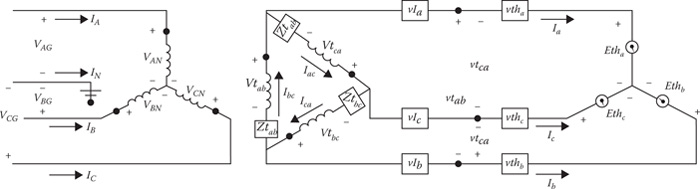
FIGURE 9.13
Ungrounded wye–delta with secondary connected to induction motor.

images

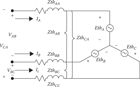
FIGURE 9.14
Primary Thevenin circuit.

$[Z_{l}_{_{a b c}}] = [\begin{matrix} Z_{l}_{_{a a}} & Z_{l}_{_{a b}} & Z_{l}_{_{a c}} \\ Z_{l}_{_{b a}} & Z_{l}_{_{b b}} & Z_{l}_{_{b c}} \\ Z_{l}_{_{c a}} & Z_{l}_{_{c b}} & Z_{l}_{_{c c}} \end{matrix}]$ (9.75)

The ungrounded wye–delta connected transformer per-unit impedance converted to actual impedance is ohms referenced to the delta-connected secondary terminals are:

$[Z t_{a b c}] = [\begin{matrix} Z t_{a b} & 0 & 0 \\ 0 & Z t_{b c} & 0 \\ 0 & 0 & Z t_{c a} \end{matrix}]$ (9.76)

The voltage drops including the secondary lines and the motor are:

$[v_{a b c}] = [Z_{eq}_{_{a b c}}] \cdot [I_{a b c}]$ (9.77)

The line-to-line voltages at the secondary terminals of the transformer bank are:

$\begin{array}{l} [\begin{matrix} V_{a b} \\ V_{b c} \\ V_{c a} \end{matrix}] = [\begin{matrix} E_{t h}_{_{a}} - E_{t h}_{_{b}} \\ E_{t h}_{_{b}} - E_{t h}_{_{c}} \\ E_{t h}_{_{c a}} - E_{t h}_{_{a}} \end{matrix}] + [\begin{matrix} v_{a} - v_{b} \\ v_{b} - v_{c} \\ v_{c} - v_{a} \end{matrix}] \\ [V_{L L}_{_{a b c}}] = [D v] \cdot [E_{t h}_{_{a b c}}] + [D v] \cdot [Z_{eq}_{_{a b c}}] \cdot [I_{a b c}] \\ [V_{L L}_{_{a b c}}] = [E_{t h} {_{_{L L}}}_{_{_{a b c}}}] + [Z_{eq}_{_{L L}}] \cdot [I_{a b c}] \end{array}$ (9.78)

where

$\begin{array}{l} [E_{t h} {_{_{L L}}}_{_{_{a b c}}}] = [D v] \cdot [E_{t h}_{_{a b c}}] \\ [Z_{eq}_{_{L L}}] = [D v] \cdot [Z_{eq}_{_{a b c}}] \end{array}$

The primary currents are:

$[I_{A B C}] = [\begin{matrix} I_{A} \\ I_{B} \\ I_{C} \end{matrix}]$ (9.79)

In Chapter 8, the currents flowing inside the delta secondary windings were defined as:

$[I_{D}_{_{a b c}}] = {[A I]}^{- 1} \cdot [I_{A B C}]$ (9.80)

where

$\begin{array}{l} [I_{D}_{_{a b c}}] = [\begin{matrix} I_{b a} \\ I_{c b} \\ I_{c a} \end{matrix}] \\ [A I] = \frac{1}{n_{t}} \cdot [\begin{matrix} 1 & 0 & 0 \\ 0 & 1 & 0 \\ 0 & 0 & 1 \end{matrix}] \\ n_{t} = \frac{k V_{L N}_{_{high}}}{k V_{L L}_{_{low}}} \end{array}$

The secondary line currents as a function of the primary line currents are:

$\begin{array}{l} [I_{a b c}] = [D i] \cdot [I_{D}_{_{a b c}}] \\ [I_{a b c}] = [D i] \cdot {[A I]}^{- 1} \cdot [I_{A B C}] \end{array}$ (9.81)

where

$[D i] = [\begin{matrix} 1 & 0 & - 1 \\ - 1 & 1 & 0 \\ 0 & - 1 & 1 \end{matrix}]$

Substitute Equation 9.81 into Equation 9.78:

$\begin{array}{l} [V_{L L}_{_{a b c}}] = [E_{t h} {_{_{L L}}}_{_{_{a b c}}}] + [Z_{eq}_{_{L L}}] \cdot [I_{a b c}] \\ [I_{a b c}] = [D i] \cdot {[A I]}^{- 1} \cdot [I_{A B C}] \\ [V_{L L}_{_{a b c}}] = [E_{t h} {_{_{L L}}}_{_{_{a b c}}}] + [Z_{eq}_{_{L L}}] \cdot [D i] \cdot {[A I]}^{- 1} \cdot [I_{A B C}] \end{array}$ (9.82)

The voltage across the transformer secondary windings are:

$\begin{array}{l} [\begin{matrix} V_{t}_{_{a b}} \\ V_{_{t}}_{_{_{b c}}} \\ V_{t}_{_{c a}} \end{matrix}] = [\begin{matrix} V_{a b} \\ V_{b c} \\ V_{c a} \end{matrix}] + [\begin{matrix} Z_{t}_{_{a b}} & 0 & 0 \\ 0 & Z_{t}_{_{b c}} & 0 \\ 0 & 0 & Z_{t}_{_{c a}} \end{matrix}] \cdot [\begin{matrix} I_{a b} \\ I_{b c} \\ I_{c a} \end{matrix}] \\ [V_{t}_{_{a b c}}] = [V_{L L}_{_{a b c}}] + [Z_{t}_{_{a b c}}] \cdot [I_{D}_{_{a b c}}] \\ [V_{t}_{_{a b c}}] = [V_{L L}_{_{a b c}}] + [Z_{t}_{_{a b c}}] \cdot {[A I]}^{- 1} \cdot [I_{A B C}] \end{array}$ (9.83)

Substitute Equation 9.82 into Equation 9.83:

$\begin{array}{l} [V_{t}_{_{a b c}}] = [V_{L L}_{_{a b c}}] + [Z_{t}_{_{a b c}}] \cdot {[A I]}^{- 1} \cdot [I_{A B C}] \\ [V_{L L}_{_{a b c}}] = [E_{t h} {_{_{L L}}}_{_{_{a b c}}}] + [Z_{eq}_{_{L L}}] \cdot [D i] \cdot {[A I]}^{- 1} \cdot [I_{A B C}] \\ [V_{t}_{_{a b c}}] = ([E_{t h} {_{_{L L}}}_{_{_{a b c}}}] + [Z_{eq}_{_{L L}}] \cdot [D i] \cdot {[A I]}^{- 1} \cdot [I_{A B C}]) + [Z_{t}_{_{a b c}}] \cdot [A I] \cdot [I_{A B C}] \\ [V_{t}_{_{a b c}}] = [E_{t h} {_{_{L L}}}_{_{_{a b c}}}] + ([Z_{eq}_{_{L L}}] \cdot [D i] + [Z_{t}_{_{a b c}}]) \cdot [A I^{- 1}] \cdot [I_{A B C}] \end{array}$ (9.84)

The primary line-to-neutral voltages are:

$\begin{array}{l} [V_{L N}_{_{A B C}}] = [A V] \cdot [V_{t}_{_{a b c}}] \\ [V_{t}_{_{a b c}}] = [E_{t h} {_{_{L L}}}_{_{_{a b c}}}] + ([Z_{eq}_{_{L L}}] \cdot [D i] + [Z_{t}_{_{a b c}}]) \cdot {[A I]}^{- 1} \cdot [I_{A B C}] \\ [V_{L N}_{_{A B C}}] = [A V] \cdot ([E_{t h} {_{_{L L}}}_{_{_{a b c}}}] + ([Z_{eq}_{_{L L}}] \cdot [D i] + [Z_{t}_{_{a b c}}]) \cdot {[A I]}^{- 1} \cdot [I_{A B C}]) \\ [V_{L N}_{_{A B C}}] = [A V] \cdot [E_{t h} {_{_{L L}}}_{_{_{a b c}}}] + [A V] \cdot ([Z_{eq}_{_{L L}}] \cdot [D i] + [Z_{t}_{_{a b c}}]) \cdot {[A I]}^{- 1} \cdot [I_{A B C}] \\ but: [E_{t h} {_{_{L L}}}_{_{_{a b c}}}] = [D v] \cdot [E_{t h}_{_{a b c}}] \\ [Z_{eq}_{_{L L}}] = [D v] \cdot [Z_{eq}_{_{a b c}}] \\ [V_{L N}_{_{A B C}}] = [A V] \cdot [D v] \cdot [E_{t h}_{_{a b c}}] + [A V] \cdot ([D v] \cdot [Z_{eq}_{_{a b c}}] \cdot [D i] + [Z_{t}_{_{a b c}}]) \cdot {[A I]}^{- 1} \cdot [I_{A B C}] \\ [V_{L N}_{_{A B C}}] = [E_{t h}_{_{A B C}}] + [Z_{t}_{_{A B C}}] \cdot [I_{A B C}] \end{array}$ (9.85)

where

$\begin{array}{l} [E_{t h}_{_{A B C}}] = [A V] \cdot [D v] \cdot [E_{t h}_{_{a b c}}] \\ [Z_{t h}_{_{A B C}}] = [A V] \cdot ([D v] \cdot [Z_{eq}_{_{a b c}}] \cdot [D i] + [Z_{t h}_{_{a b c}}]) \cdot {[A I]}^{- 1} \end{array}$

Example 9.10

For the system in Figure 9.13, the ungrounded wye–delta transformer bank consists of three single-phase transformers each rated:

50 kVA, 7200/480 V, Z_t = 0.011 + j0.018 per-unit

The impedance matrix for the transformer bank relative to the 480-V side is:

$[Z_{t}_{_{a b c}}] = [\begin{matrix} 0.0507 + j 0.0829 & 0 & 0 \\ 0 & 0.0507 + j 0.0829 & 0 \\ 0 & 0 & 0.0507 + j 0.0829 \end{matrix}] Ω$

The secondary in the system is a triplex cable of 500 ft long. The impedance matrix for the cable is:

$[Z_{l}_{_{a b c}}] = [\begin{matrix} 0.1140 + j 0.4015 & 0.0271 + j 0.2974 & 0.0271 + j 0.2735 \\ 0.0271 + j 0.2974 & 0.1140 + j 0.4015 & 0.0271 + j 0.2974 \\ 0.0271 + j 0.2735 & 0.0271 + j 0.2974 & 0.1140 + j 0.4015 \end{matrix}] Ω$

The induction motor is the motor from Example 9.9 operating at a slip of 0.035. The line-to-line voltages at the primary terminals of the transformer bank are:

$[V_{L L}_{_{A B C}}] = [\begin{matrix} 12470 \underset{____}{/ 0} \\ 11850 \underset{____}{/ - 118} \\ 12537 \underset{____}{/ 123.4} \end{matrix}] V$

Determine the Thevenin equivalent circuit of Figure 9.13 relative to the primary side of the transformer bank.Step : Because the system conditions have changed, it is necessary to run a power-flow program to determine the motor stator voltages and currents. For the ungrounded wye–delta transformer bank, the equivalent line-to-neutral voltages must first be computed.

$[V_{L N}_{_{A B C}}] = [W] \cdot [V_{L L}_{_{A B C}}] = [\begin{matrix} 7340.4 \underset{____}{/ - 28.4} \\ 6949.6 \underset{____}{/ - 149.9} \\ 6989.6 \underset{____}{/ 93.7} \end{matrix}] V$

A simple Mathcad routine was run to compute the stator and rotor voltages and currents with the following results:

$\begin{array}{l} [V_{s}_{_{a b c}}] = [\begin{matrix} 258.1 \underset{____}{/ - 58.3} \\ 259.9 \underset{____}{/ - 179.0} \\ 250.8 \underset{____}{/ 59.9} \end{matrix}] [V_{r}_{_{a b c}}] = [\begin{matrix} 224.9 \underset{____}{/ - 68.3} \\ 225.7 \underset{____}{/ 171.6} \\ 227.1 \underset{____}{/ 51.6} \end{matrix}] V \\ [I_{s}_{_{a b c}}] = [\begin{matrix} 118.9 /____- 85.7____ \\ 106.6 \underset{____}{/ 143.2} \\ 94.1 /____35.6____ \end{matrix}] [I_{r}_{_{a b c}}] = [\begin{matrix} 110.4 \underset{____}{/ - 67.3} \\ 92.2 \underset{____}{/ 163.6} \\ 88.6 \underset{____}{/ 58.8} \end{matrix}] A \end{array}$

The total three-phase converted power is:

$S_{r}_{_{a b c}} = \sum_{k = 1}^{3} \frac{V_{r}_{{_{a b c}}_{_{k}}} \cdot I_{r} {_{{_{a b c}}_{_{k}}}}^{*}}{1000} = 65.4 kW$

The ABCD matrices for the motor are those computed in Example 9.6. The Thevenin equivalent voltages and currents are:

$\begin{array}{l} [E_{t h}_{_{a b c}}] = ([A_{m}_{_{a b c}}] - [B_{m}_{_{a b c}}] \cdot {[D_{m}_{_{a b c}}]}^{- 1} \cdot [C_{m}_{_{a b c}}]) \cdot V_{r}_{_{a b c}} = [\begin{matrix} 218.7 \underset{____}{/ - 67.4} \\ 219.5 \underset{____}{/ 172.4} \\ 220.9 \underset{____}{/ 52.3} \end{matrix}] \\ [Z_{t h}_{_{a b c}}] = [B_{m}_{_{a b c}}] \cdot {[D_{m}_{_{a b c}}]}^{- 1} = [\begin{matrix} 0.1202 + j 0.2808 & - 0.0601 - j 0.1404 & - 0.0601 - j 0.1404 \\ - 0.0601 - j 0.1404 & 0.1202 + j 0.2808 & - 0.0601 - j 0.1404 \\ - 0.0601 - j 0.1404 & - 0.0601 - j 0.1404 & 0.1202 + j 0.2808 \end{matrix}] \end{array}$

It is always a good practice to confirm that the Thevenin equivalent voltages and currents will give the same stator line-to-neutral voltages that were computed at the end of the power-flow program.

$[V_{s}_{_{a b c}}] = [E_{t h}_{_{a b c}}] + [Z_{t h}_{_{a b c}}] \cdot [I_{s}_{_{a b c}}] = [\begin{matrix} 258.1 \underset{____}{/ - 58.3} \\ 259.9 \underset{____}{/ - 179.0} \\ 250.8 \underset{____}{/ 59.9} \end{matrix}]$

These voltages match those from the power-flow program, which confirms the accuracy of the Thevenin equivalent circuit for the motor.From Equations 9.78 and 9.85, the Thevenin equivalent voltages and currents on the primary side of the transformer bank are:

$\begin{array}{l} [E_{t h}_{_{A B C}}] = [A V] \cdot [D v] \cdot [E_{t h}_{_{a b c}}] = [\begin{matrix} 5699.3 \underset{____}{/ - 37.4} \\ 5722.9 \underset{____}{/ - 157.5} \\ 5702.8 \underset{____}{/ 82.3} \end{matrix}] \\ [Z_{t h}_{_{A B C}}] = [\begin{matrix} 131.7 + j 255.0 & - 60.1 - j 112.8 & - 60.1 - j 123.6 \\ - 60.1 - j 112.8 & 131.7 + j 255.0 & - 60.1 - j 123.6 \\ - 60.1 - j 123.6 & - 60.1 - j 123.6 & 131.7 + j 265.8 \end{matrix}] \end{array}$

Check to confirm that the Thevenin voltages and currents give the initial values of the primary line-to-neutral voltages at the start of the power-flow program.

$\begin{array}{l} [V_{L N}_{_{A B C}}] = [E_{t h}_{_{A B C}}] + [Z_{t h}_{_{A B C}}] \cdot [I_{A B C}] \\ [V_{L N}_{_{A B C}}] = [\begin{matrix} 7340.4 \underset{____}{/ - 28.4} \\ 6949.6 \underset{____}{/ - 149.9} \\ 6989.6 \underset{____}{/ 93.7} \end{matrix}] \end{array}$

These exactly match the initial LN transformer voltages.

9.6 Summary

This chapter has developed load models for typical loads on a distribution feeder. It is important to recognize that a combination of constant PW, constant Z, and constant current loads can be modeled using a percentage of each model. An extended model for a three-phase induction machine has been developed with examples of the machine operating as a motor and as a generator. An iterative procedure for the computation of slip to force the input power to the machine to be a specified value was developed and used in examples for both a motor and a generator. Thevenin equivalent circuits have been developed for an induction motor. The Thevenin circuit is used to develop a Thevenin equivalent circuit at the primary terminals of the step-down transformer feeding the secondary and the induction motor. This final Thevenin circuit is used in Chapter 10 on short-circuit analysis.

Problems

9.1 A 12.47-kV feeder provides service to an unbalanced wye-connected load specified to be:

Phase a: 1000 kVA, 0.9 lagging power factor
Phase b: 800 kVA, 0.95 lagging power factor
Phase c: 1100 kVA, 0.85 lagging power factor

Compute the initial load currents, assuming the loads are modeled as constant complex power.
Compute the magnitude of the load currents that will be held constant, assuming the loads are modeled as constant current.
Compute the impedance of the load to be held constant, assuming the loads are modeled as constant impedance.
Compute the initial load currents, assuming that 60% of the load is complex power, 25% constant current, and 15% constant impedance.

9.2 Using the results of Problem 9.1, rework the problem at the start of the second iteration if the load voltages after the first iteration have been computed to be:

$[V_{L N}_{_{a b c}}] = [\begin{matrix} 6851 \underset{____}{/ - 1.9} \\ 6973 \underset{____}{/ - 122.1} \\ 6886 \underset{____}{/ 117.5} \end{matrix}] V$

9.3 A 12.47-kV feeder provides service to an unbalanced delta-connected load specified to be:

Phase a: 1500 kVA, 0.95 lagging power factor
Phase b: 1000 kVA, 0.85 lagging power factor
Phase c: 950 kVA, 0.9 lagging power factor

Compute the load and line currents if the load is modeled as constant complex power.
Compute the magnitude of the load current to be held constant if the load is modeled as constant current.
Compute the impedance to be held constant if the load is modeled as constant impedance.
Compute the line currents if the load is modeled as 25% constant complex power, 20% constant current, and 55% constant impedance.

9.4 After the first iteration of the system in Problem 9.5, the load voltages are:

$[V_{L L}_{_{a b c}}] = [\begin{matrix} 11, 981 \underset{____}{/ 28.3} \\ 12, 032 \underset{____}{/ - 92.5} \\ 11, 857 \underset{____}{/ 147.7} \end{matrix}] V$

Compute the load and line currents if the load is modeled as constant complex power.
Compute the load and line currents if the load is modeled as constant current.
Compute the load and line current if the load is modeled as constant impedance.
Compute the line currents if the load mix is 25% constant complex power, 20% constant current, and 55% constant impedance.

9.5 A three-phase induction motor has the following data:

25 Hp, 240 V
Z_s = 0.0336 + j0.08 pu
Z_r = 0.0395 + j0.08 pu
Z_m = j3.12 pu

The motor is operating with a slip of 0.03 with balanced three-phase voltages of 240 V line-to-line. Determine the following:

The input line currents and complex three-phase input complex power
The currents in the rotor circuit
The developed shaft power in HP

9.6 The motor in Problem 9.5 is operating with a slip of 0.03, and the line-to-

line voltage magnitudes are:

$V_{a b} = \underset{____}{240}, V_{b c} = 230, V_{c a} = 250 V$

Compute the angles for the line-to-line voltages assuming the voltage a–b is reference.
For the given voltages and slip, determine the input line currents and complex input complex power.
Compute the rotor currents.
Compute the developed shaft power in HP.

9.7 The motor of Problem 9.5 is operating with line-to-line voltages of:

$V_{a b} = 240 \underset{__}{/ 0}, V_{b c} = 233.4 \underset{____}{/ - 118.1}, V_{c a} = 240 \underset{____}{/ 122.1} V$

The motor input kW is to be 20 kW.

Determine the following:

Required slip
The input kW and kvar
The converted shaft power

9.8 A three-phase 100-hp, 480 V wye-connected induction motor has the following per-unit impedances:

$Z_{pu}_{_{s}} = 0.043 + j 0.089, Z_{pu}_{_{r}} = 0.034 + j 0.081, Z_{pu}_{_{m}} = j 3.11$

The rotating loss is P_FW = 275 kW

Determine the impedances in ohms.
The motor is operating with a slip of 0.035. Determine the input shunt admittance matrix [YM_abc.

9.9 The motor in Problem 9.8 is operating at a slip of 0.035 with line-to-line input voltages of:

$[V_{L L}_{_{a b c}}] = [\begin{matrix} V_{a b} \\ V_{b c} \\ V_{c a} \end{matrix}] = [\begin{matrix} 480.0 \underset{____}{/ 0} \\ 475.0 \underset{____}{/ - 121.5} \\ 466.7 \underset{____}{/ 119.8} \end{matrix}]$

Determine the following:

The input stator currents
The per-phase complex input power
The total three-phase complex input power
The stator voltage and current unbalances

9.10 For the motor in Problem 9.8, determine:

For the T equivalent circuit, the matrices

$[A m_{a b c}], [B m_{a b c}], [C m_{a b c}], [D m_{a b c}]$
For the results in Problem 9.9, determine:
1. The rotor currents and output voltages
2. The rotor converted and shaft powers
3. Rotor and stator “copper” losses

9.11 For the induction motor in Problem 9.8, determine the value of the positive sequence slip that will develop 75 kW of input power to the motor.

9.12 The induction motor in Problem 9.9 is operating as a generator with a positive sequence slip of −0.04. Determine the stator output complex power.

9.13 Using the results of Problem 9.10, determine the line-to-line motor Thevenin voltages and Thevenin equivalent matrix.

9.14 The motor in Problem 9.8 is connected through a three-phase distribution line to three single-phase transformers as shown in Figure 9.15.

The three-phase induction motor is that of Problem 9.8. The secondary impedance matrix is:

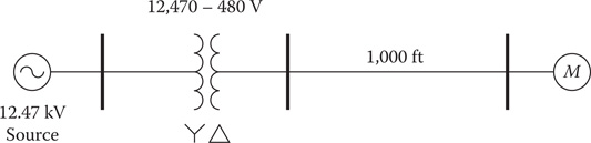
$[z_{l}_{_{a b c}}] = [\begin{matrix} 0.4013 + j 1.4133 & 0.0953 + j 1.0468 & 0.0953 + j 0.9627 \\ 0.0953 + j 1.0468 & 0.4013 + j 1.4133 & 0.0953 + j 1.0468 \\ 0.0953 + j 0.9627 & 0.0953 + j 1.0468 & 0.4013 + j 1.4133 \end{matrix}] Ω /mile$

images

FIGURE 9.15
Simple system.

The three-phase transformer bank consists of three single-phase transformers each rated:

$k V A = 100, k V_{L N}_{_{h i}} = 7.2, k V_{L L}_{_{low}} = 0.48, Z_{pu} = 0.0133 + j 0.019$

The motor is operating at a slip of 0.035.

Determine the Thevenin equivalent line-to-neutral voltages referenced to the high-voltage side of the transformers [Eth_ABC] and Thevenin equivalent line impedance matrix [Zth_ABC].

References

1. Kersting, W. H. and Phillips, W. H., Phase frame analysis of the effects of voltage unbalance on induction machines, IEEE Transactions on Industry Applications, Vol. 33, pp. 415–420, 1997.

2. American national standard for electric power systems and equipment– Voltage ratings (60 Hertz), ANSI C84.1-1995, National Electrical Manufacturers Association, Rosslyn, Virginia, 1996.

..................Content has been hidden....................

You can't read the all page of ebook, please click here login for view all page.

Table of Contents for 9. Load Models

Create new playlist

Sign In

Sign Up

9Load Models

9.1 Wye-Connected Loads

9.1.1 Constant Real and Reactive Power Loads

9.1.2 Constant Impedance Loads

9.1.3 Constant Current Loads

9.1.4 Combination Loads

Example 9.1

9.2 Delta-Connected Loads

9.2.1 Constant Real and Reactive Power Loads

9.2.2 Constant Impedance Loads

9.2.3 Constant Current Loads

9.2.4 Combination Loads

9.2.5 Line Currents Serving a Delta-Connected Load

9.3 Two-Phase and Single-Phase Loads

9.4 Shunt Capacitors

9.4.1 Wye-Connected Capacitor Bank

9.4.2 Delta-Connected Capacitor Bank

9.5 Three-Phase Induction Machine

9.5.1 Induction Machine Model

Example 9.2

9.5.2 Symmetrical Component Analysis of a Motor

Example 9.3

9.5.3 Phase Analysis of an Induction Motor [1]

Example 9.4

9.5.4 Voltage and Current Unbalance [2]

Example 9.5

9.5.5 Motor Starting Current

9.5.6 The Equivalent T Circuit

Example 9.6

9.5.7 Computation of Slip

Example 9.7

9.5.8 Induction Generator

Example 9.8

9.5.9 Induction Machine Thevenin Equivalent Circuit

Example 9.9

9.5.10 The Ungrounded Wye–Delta Transformer Bank with an Induction Motor

Example 9.10

9.6 Summary

Problems

References

Table of Contents for
9. Load Models

9
Load Models