Chapter 2
Using the Excel Interface

Using the Ribbon

The mantra of the ribbon is to use pictures and words. Many people noticed the little whisk broom icon in previous versions of Excel but never knew what it did. In the ribbon, the same icon has the words “Format Painter” next to it. When you hover, the ToolTip offers paragraphs explaining what the tool does. The ToolTip also offers a little-known trick: You can double-click the Format Painter to copy the formatting to many places.

The Look of the Ribbon Is Changing

In early 2007, all of Office moved from a menu bar to the ribbon. At first, the ribbon was super confusing. You would constantly be hunting from ribbon tab to ribbon tab trying to find where the command you needed was hiding. For example:

• In Excel 2003, Insert Rows was on the Insert menu, but in Excel 2007, Insert Rows was on the far-right side of the Home tab.

• Pivot Tables, which had been on the Data menu, were moved to the Insert tab.

• The ribbon was taller than the combination of the menu, the Standard Toolbar, and the Formatting Toolbar, which meant that you could see a few less rows in your Excel worksheet.

After 20 minutes of struggling with the new ribbon in 2007, you were finally ready to Print, Save, or Send, but the File tab was not there. Microsoft had replaced the word “File” with an Office logo that few people thought to click. When you clicked the Office logo, the File menu opened.

Most who used Excel 2003 for 40 hours a week hated the new ribbon at first. I remember dedicating every Wednesday of my MrExcel Podcast to a new feature called “Where Is It Wednesday.” A new theme song for the Wednesday podcast had a lyric that said, “It’s a great feature, I just can’t find it anymore.”

Even Bill Gates asked, “You are going to offer a classic mode, right?” But somehow, Jensen Harris and the Office User Interface team convinced Bill Gates that there should be no classic mode.

The ribbon improved slightly in Office 2010. The Office logo in the top left was replaced with the word “File.” Hardcore Excel users eventually figured out where their favorite features were located.

And now, Microsoft is talking about changing the ribbon again. They say the ribbon is too tall and it gets in the way. They are talking about a special mode where the ribbon will be a single row. Also, they want to use less color in the ribbon.

The great news for Excel users is that the new ribbon is first being added to Outlook, and then it will be added to the online version of Excel. The core Excel, Word, and PowerPoint running on client computers will not get the one-row ribbon until Microsoft gauges the reaction to the shorter ribbon in Outlook and Excel Online.

Most people do not use Excel online, so the new ribbon won’t bother us.

Even if we don’t get the one-row ribbon soon, Microsoft is still changing the look of the tall ribbon, but only for Office 365 customers.

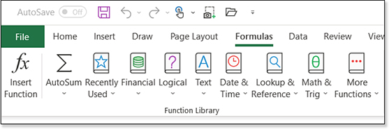
Figure 2.1 shows the new ribbon that started rolling out to Office 365 customers in the Summer of 2018. One big change is the active ribbon tab is denoted with a horizontal line instead of a block of color. In Figure 2.1, the word “Formulas” is underlined. Also, the new ribbon uses less color. The icons look like line art instead of the rich illustrations of the past.

Contrast the new ribbon above with the Excel 2019 ribbon in Figure 2.2.

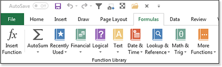
Many people hate change; I like the old ribbon better. In the old ribbon, the Logical icon looked like a purple hard-bound book; the book’s spine was on the left, and the icon had some depth, which made it look like a book. Because the icons now use less color, the same icon in Office 365 uses black lines to try to indicate a book. The spine is not obvious, the depth is fainter, and it doesn’t look as much like a book anymore.

Microsoft started using the new ribbon in Office 365 in mid-2018, which means anyone who purchases the perpetual Excel 2019 will be stuck with the old ribbon. I do not understand the hostile attitude of Microsoft Marketing to their perpetual edition customers. It is as if they are saying, “Thank you for your $400. We are going to give you an inferior, out-of-date product to punish you for refusing to switch to our $10-a-month subscription plan.”

If someone bought the perpetual Office 2016 on January 30, 2016, they would have paid $400. Another customer purchasing Office 365 on January 20, 2016 would have paid $10 a month or about $320 by the time Office 2019 is released in the fall of 2018. The perpetual edition customers are paying more than the Office 365 customers, and Microsoft is blatantly treating them like second-class citizens.

The title on the front cover of this book is “Excel 2019 Inside Out,” so I will be using the old-style Excel 2019 ribbon in the screenshots for this book. But there is a good chance that you are using Office 365 and have the new style ribbon. Luckily, the same commands appear in the same sequence. Your icons simply have less color.

Using Flyout Menus and Galleries

One element in the ribbon is the gallery control. Galleries are used when there are dozens of options from which you can choose. The gallery shows you a visual thumbnail of each choice. A gallery starts out showing a row or two of choices in the ribbon. (For an example, open the Cell Styles gallery on the Excel 2019 Home tab.) The right side of the gallery offers icons for Up, Down, and Open. If you click Up or Down, you scroll one row at a time through the choices.

If you click the Open control at the bottom-right side of the gallery, the gallery opens to reveal all choices at once.

Rolling Through the Ribbon Tabs

With Excel as the active application, move the mouse anywhere over the ribbon and roll the scroll wheel on top of the mouse. Excel quickly flips from tab to tab on the ribbon. Scroll away from you to roll toward the Home tab on the left. Scroll toward you to move to the right.

Revealing More Commands Using Dialog Box Launchers, Task Panes, and “More” Commands

The ribbon holds perhaps 20 percent of the available commands. The set of commands and options available in the ribbon will be enough 80 percent of the time, but you will sometimes have to go beyond the commands in the ribbon. You can do this with dialog box launchers, More commands, and the task pane.

A dialog box launcher is a special symbol in the lower-right corner of many ribbon groups. Click the dialog box launcher to open a related dialog box with many more choices than those offered in the ribbon.

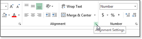
Figure 2.3 shows details of the Alignment group of the Home tab. In the lower-right corner of the group is the dialog box launcher. It looks like the top-left corner of a dialog box, with an arrow pointing downward and to the right.

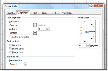
When you click the dialog box launcher, you go to a dialog box that often offers many more choices than those available in the ribbon. In Figure 2.4, you see the Alignment tab of the Format Cells dialog box.

Many menus in the ribbon end with an entry for finding more rules and option; these entries end with an ellipsis (…). Clicking a More item takes you to a dialog box or task pane with more choices than those available in the ribbon.

Resizing Excel Changes the Ribbon

The ribbon modifies as the size of the Excel application window changes. You should be aware of this when you are coaching a co-worker over the phone. You might be looking at your screen and telling him to “look for the big Insert drop-down menu to the right of the orange word Calculation.” Although this makes perfect sense on your widescreen monitor, it might not make sense on his monitor. Figure 2.5 shows some detail of the Home tab on a widescreen monitor. The Cell Styles gallery shows ten thumbnails, and Insert, Delete, and Format appear side-by-side.

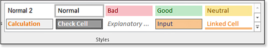
Figure 2.6 shows the typical view on a laptop. The Cell Styles gallery is collapsed to a single drop-down menu. The Insert, Delete, and Format icons are now arranged vertically.

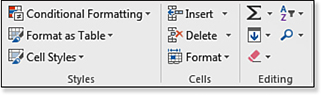
As you resize the Excel screen to a smaller width, more items collapse. Soon, the three icons for Insert, Delete, and Format are collapsed into a single drop-down menu called Cells. Eventually, the Excel ribbon gets too small, and Excel hides it completely.

Activating the Developer Tab

If you regularly record or write macros, you might be looking for the VBA tools in the ribbon. They are all located on the Developer tab, which is hidden by default. However, it is easy to make the Developer tab visible. Follow these steps:

1. Right-click the ribbon and choose Customize The Ribbon. Excel displays the Customize Ribbon category of the Excel Options dialog box.

2. A long list box of ribbon tabs is shown on the right side of the screen. Every one of them is checked except for Developer. Check the box next to Developer.

3. Click OK. The Developer tab displays.

Activating Contextual Ribbon Tabs

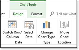
The ribbon tabs you see all the time are called the main tabs. Another 23 tabs come and go, depending on what is selected in Excel. In Figure 2.7, you can see two contextual tabs that appear only when a chart is selected.

Here is the frustrating thing: As soon as you click outside of the object (that is, the chart), it is no longer selected, and the Chart Tools tabs disappear.

If you need to format an object and you cannot find the icons for formatting it, try clicking the object to see if the contextual tabs appear.

Two other tabs occasionally appear, although Excel classifies them as main tabs instead of contextual tabs. If you add the Print Preview Full Screen icon to the interface, you arrive at a Print Preview tab. Also, from the Picture Tools Design tab, you can click Remove Background to end up at the Background Removal tab.

Finding Lost Commands on the Ribbon

Often, the command you need is front and center on the Home tab, and everything is fine. However, there are times when you cannot find an obscure command that you know is somewhere in Excel.

Microsoft introduced a new Tell Me What You Want to Do search box on the Office 2016 ribbon. The functionality of that box has improved for Excel 2019.

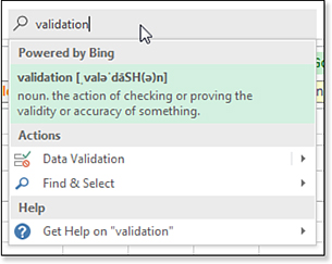
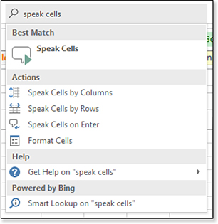
Type Validation in the box. The results are shown in Figure 2.8. They define the term for you. They tell you how to pronounce the word. They offer the Data Validation command. They offer Help on the command. It works well. For some reason, they offer the Find & Select command as well, but you can overlook that.

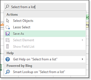
This feature works okay if you know the name of the command that you are searching for. If you try to answer the Tell Me What You Want To Do box with an English language phrase, such as Choose from a list, the search box has little chance of returning the command (see Figure 2.9). I’ve tested many phrases and never get the command that I am describing.

One great improvement since Excel 2016: If you know the name of the command but the command falls into the dreaded “commands not in ribbon” category, the Search box will successfully return the command and offer you a way to invoke it (see Figure 2.10).

Here is my strategy for finding those commands that aren’t on the ribbon:

1. Right-click the ribbon and select Customize Quick Access Toolbar. Excel displays the Quick Access Toolbar category of the Excel Options dialog box.

2. Open the top-left drop-down menu and change Popular Commands to All Commands. You now have an alphabetical list of more than 2,000 commands.

3. Scroll through this alphabetical list until you find the command you are trying to locate in the ribbon.

4. Hover over the command in the left list box. A ToolTip appears, showing you where you can find the command. If the ToolTip shows Command Not In Ribbon, click the Add button in the center of the screen to add the command to the Quick Access Toolbar.

Shrinking the Ribbon

The ribbon takes up four vertical rows of space. This won’t be an issue on a big monitor, but it could be an issue on a tiny laptop.

To shrink the ribbon, you can right-click it and choose Collapse The Ribbon. Or, use the carat (^) icon on the far-right side of the ribbon. The ribbon collapses to show only the ribbon tabs. When you click a tab, the ribbon temporarily expands. To close the ribbon, choose a command or press Esc.

To permanently bring the ribbon back to full size, right-click a ribbon tab and uncheck Collapse The Ribbon. Or, click any tab and then click the pushpin icon in the lower-right corner of the ribbon. You can also toggle between minimized and full size by double-clicking any ribbon tab.

Using the Quick Access Toolbar

A problem with the ribbon is that only one-seventh of the commands are visible at any given time. You will find yourself moving from one tab to another. The alternative is to use the Quick Access Toolbar (QAT) to store your favorite commands.

The QAT starts out as a tiny toolbar with AutoSave, Save, Undo, and Redo. It is initially located above the File tab in the ribbon.

If you start using the QAT frequently, you can right-click the toolbar and choose Show Quick Access Toolbar Below The Ribbon to move the QAT closer to the grid.

Adding Icons to the QAT

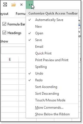
The drop-down menu at the right side of the QAT, shown on the right side in Figure 2.11, offers 12 popular commands you might choose to add to the Quick Access Toolbar. Choose a command from this list to add it to the QAT.

When you find a command in the ribbon you are likely to use often, you can easily add the command to the QAT. To do so, right-click any command in the ribbon and select Add To Quick Access Toolbar. Items added to the Quick Access Toolbar using the right-click method are added to the right side of the QAT.

The right-click method works for many commands, but not with individual items within commands. For example, you can put the Font Size drop-down menu on the QAT, but you cannot specifically put size 16 font in the QAT.

Removing Commands from the QAT

You can remove an icon from the QAT by right-clicking the icon and selecting Remove from Quick Access Toolbar.

Customizing the QAT

You can make minor changes to the QAT by using the context menus, but you can have far more control over the QAT if you use the Customize command. Right-click the QAT and select Customize Quick Access Toolbar to display the Quick Access Toolbar section of the Excel Options dialog box, as shown in Figure 2.12.

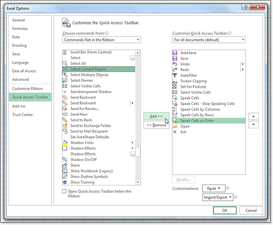
The Excel Options dialog box offers many features for customizing the Quick Access Toolbar:

• You can choose to customize the QAT for all documents on your computer or just for the current workbook by using the top-right drop-down menu.

• You can add separators between icons to group the icons logically. A separator icon is available at the top of the left menu. Click the separator icon in the left list box and then click the Add icon in the center of the screen.

• You can resequence the order of the icons on the toolbar. Select an icon in the right list box, and then click the up/down arrow icons on the right side of the dialog box.

• You can access 2,000+ commands, including the commands from every tab and commands that are not available in the ribbon. Although the dialog box starts with just 53 popular commands in the left list box, use the left drop-down menu to choose All Commands or Commands Not In The Ribbon. When you find a command in the left list box, select the command and then click Add in the center of the dialog box to add that command to the QAT.

• You can reset the QAT to its original default state using the Reset button in the lower right.

• You can export your custom QAT icons from your computer and import on another computer.

• You can move the QAT to appear above or below the ribbon using the check box in the lower left.

Using the Full-Screen File Menu

Open the File menu to see the Backstage view. Here is the logic: When you are working on most ribbon tabs, you are working in your document. When you are about to change the font or something like that, you want to see the results of the change for the “in” commands. However, the Excel team thinks that after you move to the File menu, you are done working in your document, and you are about to do something with the whole document, such as send the workbook, print the workbook, post the workbook to Twitter, and so on. Microsoft calls these the “out” commands. The theory is that you don’t need to see the worksheet for the “out” commands, so Microsoft fills the entire screen with the File menu.

To open the Backstage view, click the File menu. The Backstage view fills the screen, as shown in Figure 2.13. Backstage is split into three sections: the narrow left navigation panel and two wider sections that provide information.

The left navigation panel includes these commands:

• Home—New in Excel 2019, it combines elements of New and Open. At the top, you can see tutorials from Microsoft and popular templates. In the middle, recent and pinned files. Both sections have a link to “Find More in New” or “Find More in Open.”

• Info—Provides information about the current workbook. This is discussed later in the “Getting Information About the Current Workbook” section.

• New—Used to create a new workbook or start from a template.

• Open—Used to access a file stored on your computer or the OneDrive. See Chapter 1.

• Save—Saves the file in the same folder as it was previously stored. Note that Save is a command instead of a panel in Backstage.

• Save As—Stores the file on your computer or in OneDrive. See Chapter 1.

• Print—Used to choose print settings and print. Includes Print Preview. See Chapter 27, “Printing.”

• Share—Changed in Excel 2019. This is now the entry point for sharing a workbook with your co-workers. See Chapter 1.

• Export—Used to create a PDF or change the file type.

• Publish—Used to upload your workbook to Power BI.

• Close—Closes the current workbook. Like Save, this entry is a pure command.

• Account—Sign in to Office. Choose a color theme and a background. See if updates are available. Learn your version of Excel. This and the next two items have been moved to the bottom left of the screen, below the area shown shown in Figure 2.13.

• Feedback—Send a smile or send a frown to the Excel team. Also contains a link to the Excel.UserVoice.com website where you can suggest new ideas for Excel.

• Options—Contains pages of Excel settings. See Chapter 3, “Customizing Excel,” for details.

• Recent File List—This list appears only if you’ve changed a default setting in Excel Options. Visit File, Options, Advanced Display and choose Quickly Access This Number Of Recent Workbooks.

Pressing the Esc Key to Close Backstage View

To get out of Backstage and return to your worksheet, you can either press the Esc key or click the back arrow in the top-left corner of Backstage.

Recovering Unsaved Workbooks

As in previous versions of Excel, the AutoRecover feature can create copies of your workbook every n minutes. If you close the workbook without saving, you might be able to get the file back, provided it was open long enough to go through an AutoRecover.

If the workbook was new and never saved, scroll to the bottom of the Recent Workbooks List and choose Recover Unsaved Workbooks.

If the workbook had previously been saved, open the last saved version of the workbook. Go to the File menu, and the last AutoSave version from before you closed the file will be available.

Clearing the Recent Workbooks List

If you need to clear out the Recent Workbooks list, you should visit File, Options, Advanced, Display. Set the Show This Number Of Recent Documents list to zero. You can then set it back to a positive number, such as 10.

Getting Information About the Current Workbook

When a workbook is open, and you go to the File, Info, you see the Info gallery for that workbook. The Info pane lists all sorts of information about the current workbook:

• The workbook path is shown at the top of the center panel.

• You can see the file size.

• You can see when the document was last modified and who modified it.

• If any special states exist, these will be reported at the top of the middle pane. Special states might include the following:

  • Macros Not Enabled

  • Links Not Updated

  • Checked Out From SharePoint

• You can see if the file has been AutoRecovered and recover those versions.

• You can mark the document as final, which will cause others opening the file to initially have a read-only version of the file.

• You can edit links to other documents.

• You can add tags or categories to the file.

• Using the Check For Issues drop-down menu, you can run a compatibility checker to see if the workbook is compatible with legacy versions of Excel. You can run an accessibility checker to see if any parts of the document will be difficult for people with disabilities. You can run a Document Inspector to see if any private information is hidden in the file.

Marking a Workbook as Final to Prevent Editing

Open the Protect Workbook icon in the Info gallery to access a setting called Mark As Final. This marks the workbook as read-only. It prevents someone else from making changes to your final workbook.

However, if the other person visits the Info gallery, that person can re-enable editing. This feature is designed to warn the other people that you’ve marked it as final and no further changes should happen.

If you can convince everyone in your workgroup to sign up for a Windows Live ID, you can use the Restrict Permission By People setting. This layer of security enables you to define who can read, edit, and/or print the document.

Finding Hidden Content Using the Document Inspector

The Document Inspector can find a lot of hidden content, but it is not perfect. Still, finding 95 percent of the types of hidden content can protect you a lot of the time.

To run the Document Inspector, select File, Info, Check For Issues, Inspect Document, and click OK. The results of the Document Inspector show that the document has personal information stored in the file properties (author’s name) and perhaps a hidden worksheet.

Adding Whitespace Around Icons Using Touch Mode

If you are trying to use Excel on a tablet or a touch screen, you want to try touch mode. Follow these steps:

1. Go to the right side of the QAT and open the drop-down menu that appears there.

2. The twelfth command is called Touch/Mouse Mode. The icon is a blue dot with a ring of whitespace and then dashed lines around the whitespace. Choose this command to add it to the QAT.

3. Click the icon on the QAT. You see whitespace added around all the icons.

Using the New Sheet Icon to Add Worksheets

The Insert Worksheet icon is a circle with a plus sign that appears to the right of the last sheet tab.

When you click this icon, a new worksheet is added to the right of the active sheet. This is better than Excel 2010, where the new worksheet was added as the last worksheet in the workbook and then had to be dragged to the correct position.

Navigating Through Many Worksheets Using the Controls in the Lower Left

Older versions of Excel had four controls for moving through the list of worksheet tabs. The worksheet navigation icons are now a left and right arrowhead in the lower left.

The controls are active only when you have more tabs than are visible across the bottom of the Excel window. Click the left or right icon to scroll the tabs one at a time. Ctrl+click either arrow to scroll to the first or last tab. Note that scrolling the tabs does not change the active sheet. It just brings more tabs into view, so you can then click the selected tab.

Just as in prior versions of Excel, you can right-click the worksheet navigation arrows to see a complete list of worksheets. Click any item in the list to move to that worksheet.

In certain circumstances, an ellipsis (...) icon appears to the left of the worksheet navigation arrows. This icon selects the worksheet to the left of the active sheet.

Using the Mini Toolbar to Format Selected Text

When you select some text in a chart title or within a cell, the mini toolbar appears above the selected text. If you move away from the mini toolbar, it fades away. However, if you move the mouse toward the mini toolbar, you see several text formatting options.

To use the mini toolbar, follow these steps:

1. Select some text. If you select text in a cell, you must select a portion of the text in the cell by using Cell Edit mode. In a chart, SmartArt diagram, or text box, you can select any text. As soon as you release the mouse button, the mini toolbar appears above and to the right of the selection.

2. Move the mouse pointer toward the mini toolbar. The mini toolbar stays visible if your mouse is above it. If you move the mouse away from the mini toolbar, it fades away.

3. Make changes in the mini toolbar to affect the text you selected in step 1.

4. When you are done formatting the selected text, you can move the mouse away from the mini toolbar to dismiss it.

Expanding the Formula Bar

Formulas range from very simple to very complex. As people started writing longer and longer formulas in Excel, an annoying problem began to appear: If the formula for a selected cell was longer than the formula bar, the formula bar would wrap and extend over the worksheet. In many cases, the formula would obscure the first few rows of the worksheet. This was frustrating, especially if the selected cell was in the top few rows of the spreadsheet.

Excel 2016 includes a formula bar that prevents the formula from obscuring the spreadsheet. For example, in Figure 2.14, cell F1 contains a formula that is longer than the formula bar. Notice the down-arrow icon at the right end of the formula bar. This icon expands the formula bar.

Press Ctrl+Shift+U or click the down-arrow icon at the right side of the formula bar to expand the formula bar. The formula bar expands to the last manually resized height, and the entire worksheet moves down to accommodate the larger formula bar.

The formula, in this example, is too long for the default larger formula bar. You must hover your mouse near the bottom of the formula bar until you see the up/down white arrow cursor. Click and drag down until you can see the entire formula (see Figure 2.15).

Zooming In and Out on a Worksheet

In the lower-right corner of the Excel window, a zoom slider enables you to zoom from 400 percent to 10 percent with lightning speed. You simply drag the slider to the right to zoom in and to the left to zoom out. The Zoom Out and Zoom In buttons on either end of the slider enable you to adjust the zoom in 10 percent increments.

Clicking the % indicator to the right of the zoom slider opens the legacy Zoom dialog box.

Inside OUT

If you decrease the zoom below 40%, Microsoft assumes that you are looking for an overview of the entire spreadsheet.

An interesting feature appears when you decrease the zoom to 39% or less. Any regions that have been assigned a name will appear as boxes with the name super-imposed. This is great for getting an overview of the named ranges created by someone else.

Using the Status Bar to Add Numbers

If you select several cells that contain numeric data and then look at the status bar, at the bottom of the Excel window, you can see that the status bar reports the average, count, and sum of the selected cells (see Figure 2.16).

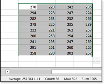
If you need to quickly add the contents of several cells, you can select the cells and look for the total in the status bar. This feature has been in Excel for a decade, yet very few people realized it was there. In legacy versions of Excel, only the sum would appear, but you could right-click the sum to see other values, such as the average, count, minimum, and maximum.

You can customize which statistics are shown in the status bar. Right-click the status bar and choose any or all of Min, Max, Numerical Count, Count, Sum, and Average.

Switching Between Normal View, Page Break Preview, and Page Layout View Modes

Three shortcut icons to the left of the zoom slider enable you to quickly switch between three view modes:

• Normal view—This mode shows worksheet cells as normal.

• Page Break preview—This mode draws the page breaks in blue. You can actually drag the page breaks to new locations in Page Break preview. This mode has been available in several versions of Excel.

• Page Layout view—This view was introduced in Excel 2007. It combines the best of Page Break preview and Print Preview modes.

In Page Layout view mode, each page is shown, along with the margins, header, and footer. A ruler appears above the pages and to the left of the pages. You can make changes in this mode in the following ways:

• To change the margins, drag the gray boxes in the ruler.

• To change column widths, drag the borders of the column headers.

• To add a header, select Click To Add Header.