Color, Shading, and Lighting
In this chapter we cover the basics of color representation, lighting models, and shading objects. Geometric modeling operations are responsible for accurately reproducing shape, size, position, and orientation. Knowledge of the basics of color, lighting, and shading are the next step in reproducing the visual appearance of an object.
3.1 Representing Color
To produce more realistic images, objects being rendered must be shaded with accurate colors. Modern graphics accelerators can faithfully generate colors from a large, but finite palette. In OpenGL, color values are specified to be represented with a triple of floating-point numbers in the range [0,1]. These values specify the amount of red, green, and blue (RGB) primaries in the color. RGB triples are also used to store pixel colors in the framebuffer, and are used by the video display hardware to drive a cathode ray tube (CRT) or liquid crystal display (LCD) display.
A given color representation scheme is referred to as a color space. The RGB space used by OpenGL is a cartesian space well suited for describing colors for display devices that emit light, such as color monitors. The addition of the three primary colors mimics the mixing of three light sources. Other examples of color spaces include:
Hue Saturation Value (HSV) model is a polar color space that is often used by artists and designers to describe colors in a more intuitive fashion. Hue specifies the spectral wavelength, saturation the proportion of the color present (higher saturation means the color is more vivid and less gray), while value specifies the overall brightness of the color.
Cyan Magenta Yellow blacK (CMYK) is a subtractive color space which mimics the process of mixing paints. Subtractive color spaces are used in publishing, since the production of colors on a printed medium involves applying ink to a substrate, which is a subtractive process. Printing colors using a mixture of four inks is called process color. In contrast, printing tasks that involve a small number of different colors may use a separate ink for each color. These are referred to as spot colors. Spot colors are frequently specified using individual codes from a color matching system such as Pantone (2003).
YCbCr is an additive color space that models colors using a brightness (Y) component and two chrominance components (Cb and Cr). Often the luminance signal is encoded with more precision than the chrominance components. YCbCr1 is used in digital video processing [Jac96].
sRGB is a non-linear color space that better matches the visual perception of brightness. sRGB serves as a standard for displaying colors on monitors (CRT and LCD) with the goal of having the same image display identically on different devices [Pac01]. Since it also matches human sensitivity to intensity, it allows colors to be more compactly or efficiently represented without introducing perceptual errors. For example, 8-bit sRGB values require 12-bit linear values to preserve accuracy across the full range of values.
The choice of an RGB color space is not critical to the functioning of the OpenGL pipeline; an application can use the rendering pipeline to perform processing on data from other color spaces if done carefully.
3.1.1 Resolution and Dynamic Range
The number of colors that can be represented, or palette size, is determined by the number of bits used to represent each of the R, G, and B color components. An accelerator that uses 8 bits per component can represent 224 (about 16 million) different colors. Color components are typically normalized to the range [0, 1], so an 8-bit color component can represent or resolve changes in [0, 1] colors by as little as 1/256. For some types of rendering algorithms it is useful to represent colors beyond the normal [0, 1] range. In particular, colors in the range [−1, 1] are useful for subtractive operations. Natively representing color values beyond the [−1, 1] range is becoming increasingly useful to support algorithms that use high dynamic range intermediate results. Such algorithms are used to achieve more realistic lighting and for algorithms that go beyond traditional rendering.
An OpenGL implementation may represent color components with different numbers of bits in different parts of the pipeline, varying both the resolution and the range. For example, the colorbuffer may store 8 bits of data per component, but for performance reasons, a texture map might store only 4 bits per component. Over time, the bit resolution has increased; ultimately most computations may well be performed with the equivalent of standard IEEE-754 32-bit floating-point arithmetic. Today, however, contemporary consumer graphics accelerators typically support 32-bit float values when operating on vertex colors and use 8 bits per component while operating on fragment (pixel) colors. Higher end hardware increases the resolution (and range) to 10, 12, or 16 bits per component for framebuffer and texture storage and as much as 32-bit floating-point for intermediate fragment computations.
Opinions vary on the subject of how much resolution is necessary, but the human eye can resolve somewhere between 10 and 14 bits per component. The sRGB representation provides a means to use fewer bits per component without adding visual artifacts. It accomplishes this using a non-linear representation related to the concept of gamma.
3.1.2 Gamma
Gamma describes the relationship between a color value and its brightness on a particular device. For images described in an RGB color space to appear visually correct, the display device should generate an output brightness directly proportional (linearly related) to the input color value. Most display devices do not have this property. Gamma correction is a technique used to compensate for the non-linear display characteristics of a device.
Gamma correction is achieved by mapping the input values through a correction function, tailored to the characteristics of the display device, before sending them to the display device. The mapping function is often implemented using a lookup table, typically using a separate table for each of the RGB color components. For a CRT display, the relationship between the input and displayed signal is approximately2 D = Iγ, as shown in Figure 3.1. Gamma correction is accomplished by sending the signal through the inverse function I1/γ as shown in Figure 3.2.
The gamma value for a CRT display is somewhat dependent on the exact characteristics of the device, but the nominal value is 2.5. The story is somewhat more complicated though, as there is a subjective aspect to the human perception of brightness (actually lightness), that is influenced by the viewing environment. CRTs are frequently used for viewing video in a dim environment. To provide a correct subjective response in this environment, video signals are typically precompensated, treating the CRT as if it has a gamma value of 2.2. Thus, the well-known 2.2 gamma value has a built-in dim viewing environment assumption [Poy98]. The sRGB space represents color values in an approximate gamma 2.2 space.
Other types of display devices have non-linear display characteristics as well, but the manufacturers typically include compensation circuits so that they appear to have a gamma of 2.5. Printers and other devices also have non-linear characteristics and these may or may not include compensation circuitry to make them compatible with monitor displays. Color management systems (CMS) attempt to solve problems with variation using transfer functions. They are controlled by a system of profiles that describes the characteristics of a device. Application or driver software uses these profiles to appropriately adjust image color values as part of the display process.
Gamma correction is not directly addressed by the OpenGL specification; it is usually part of the native windowing system in which OpenGL is embedded. Even though gamma correction isn’t part of OpenGL, it is essential to understand that the OpenGL pipeline computations work best in a linear color space, and that gamma correction typically takes place between the framebuffer and the display device. Care must be taken when importing image data into OpenGL applications, such as texture maps. If the image data has already been gamma corrected for a particular display device, then the linear computations performed in the pipeline and a second application of gamma correction may result in poorer quality images.
There are two problems that typically arise with gamma correction: not enough correction and too much correction. The first occurs when working with older graphics cards that do not provide gamma correction on framebuffer display. Uncorrected scenes will appear dark on such displays. To address this, many applications perform gamma correction themselves in an ad hoc fashion; brightening the input colors and using compensated texture maps. If the application does not compensate, then the only recourse for the user is to adjust the monitor brightness and contrast controls to brighten the image. Both of these lead to examples of the second problem, too much gamma correction. If the application has pre-compensated its colors, then the subsequent application of gamma correction by graphics hardware with gamma correction support results in overly bright images. The same problem occurs if the user has previously increased the monitor brightness to compensate for a non-gamma-aware application. This can be corrected by disabling the gamma correction in the graphics display hardware, but of course, there are still errors resulting from computations such as blending and texture filtering that assume a linear space.
In either case, the mixture of gamma-aware and unaware hardware has given rise to a set of applications and texture maps that are mismatched to hardware and leads to a great deal of confusion. While not all graphics accelerators contain gamma correction hardware, for the purposes of this book we shall assume that input colors are in a linear space and gamma correction is provided in the display subsystem.
3.1.3 Alpha
In addition to the red, green, and blue color components, OpenGL uses a fourth component called alpha in many of its color computations. Alpha is mainly used to perform blending operations between two different colors (for example, a foreground and a background color) or for modeling transparency. The role of alpha in those computations is described in Section 11.8. The alpha component also shares most of the computations of the RGB color components, so when advantageous, alpha can also be treated as an additional color component.
3.1.4 Color Index
In addition to operating on colors as RGBA tuples (usually referred to as RGB mode), OpenGL also allows applications to operate in color index mode (also called pseudo-color mode, or ramp mode). In index mode, the application supplies index values instead of RGBA tuples to OpenGL. The indexes represent colors as references into a color lookup table (also called a color map or palette). These index values are operated on by the OpenGL pipeline and stored in the framebuffer. The conversion from index to RGB color values is performed as part of display processing. Color index mode is principally used to support legacy applications written for older graphics hardware. Older hardware avoided a substantial cost burden by performing computations on and saving in framebuffer memory a single index value rather than three color components per-pixel. Of course, the savings comes at the cost of a greatly reduced color palette.
Today there are a very few reasons for applications to use color index mode. There are a few performance tricks that can be achieved by manipulating the color map rather than redrawing the scene, but for the most part the functionality of color index mode can be emulated by texture mapping with 1D texture maps. The main reason index mode is still present on modern hardware is that the native window system traditionally required it and the incremental work necessary to support it in an OpenGL implementation is usually minor.
3.2 Shading
Shading is the term used to describe the assignment of a color value to a pixel. For photorealistic applications—applications that strive to generate images that look as good as photographs of a real scene—the goal is to choose a color value that most accurately captures the color of the light reflected from the object to the viewer. Photorealistic rendering attempts to take into account the real world interactions between objects, light sources, and the environment. It describes the interactions as a set of equations that can be evaluated at each surface point on the object. For some applications, photorealistic shading is not the objective. For instance, technical illustration, cartoon rendering, and image processing all have different objectives, but still need to perform shading computations at each pixel and arrive at a color value.
The shading computation is by definition a per-pixel-fragment operation, but portions of the computation may not be performed per-pixel. Avoiding per-pixel computations is done to reduce the amount of processing power required to render a scene. Figure 3.3 illustrates schematically the places in the OpenGL pipeline where the color for a pixel fragment may be modified by parts of the shading computation.
There are five fundamental places where the fragment color can be affected: input color, vertex lighting, texturing, fog, and blending. OpenGL maintains the concept of a current color (with the caveat that it is undefined after a vertex array drawing command has been issued), so if a new color is not issued with the vertex primitive, then the current color is used. If lighting is enabled, then the vertex color is replaced with the result of the vertex lighting computation.
There is some subtlety in the vertex lighting computation. While lighting uses the current material definition to provide the color attributes for the vertex, if GL_COLOR_MATERIAL is enabled, then the current color updates the current material definition before being used in the lighting computation.3
After vertex lighting, the primitive is rasterized. Depending on the shading model (GL_FLAT or GL_SMOOTH), the resulting pixel fragments will have the color associated with the vertex or a color interpolated from multiple vertex colors. If texturing is enabled, then the color value is further modified, or even replaced altogether by texture environment processing. If fog is enabled, then the fragment color is mixed with the fog color, where the proportions of the mix are controlled by the distance of the fragment from the viewer. Finally, if blending is enabled, then the fragment color value is modified according to the enabled blending mode.
By controlling which parts of the pipeline are enabled and disabled, some simple shading models can be implemented:
Constant Shading If the OpenGL shading model is set to GL_FLAT and all other parts of the shading pipeline disabled, then each generated pixel of a primitive has the color of the provoking vertex of the primitive. The provoking vertex is a term that describes which vertex is used to define a primitive, or to delineate the individual triangles, quads, or lines within a compound primitive. In general it is the last vertex of a line, triangle, or quadrilateral (for strips and fans, the last vertex to define each line, triangle or quadrilateral within the primitive). For polygons it is the first vertex. Constant shading is also called flat or faceted shading.
Smooth Shading If the shading model is set to GL_SMOOTH, then the colors of each vertex are interpolated to produce the fragment color. This results in smooth transitions between polygons of different colors. If all of the vertex colors are the same, then smooth shading produces the same result as constant shading. If vertex lighting is combined with smooth shading, then the polygons are Gouraud shaded [Gou71].
Texture Shading If the input color and vertex lighting calculations are ignored or disabled, and the pixel color comes from simply replacing the vertex color with a color determined from a texture map, we have texture shading. With texture shading, the appearance of a polygon is determined entirely by the texture map applied to the polygon including the effects from light sources. It is quite common to decouple lighting from the texture map, for example, by combining vertex lighting with texture shading by using a GL_MODULATE texture environment with the result of computing lighting values for white vertices. In effect, the lighting computation is used to perform intensity or Lambertian shading that modulates the color from the texture map.
Phong Shading Early computer graphics papers and books have occasionally confused the definition of the lighting model (lighting) from how the lighting model is evaluated (shading). The original description of Gouraud shading applies a particular lighting model to each vertex and linearly interpolates the colors computed for each vertex to produce fragment colors. We prefer to generalize that idea to two orthogonal concepts per-vertex lighting and smooth shading. Similarly, Phong describes a more advanced lighting model that includes the effects of specular reflection. This model is evaluated at each pixel fragment to avoid artifacts that can result from evaluating the model at vertices and interpolating the colors. Again, we separate the concept of per-pixel lighting from the Phong lighting model.
In general, when Phong shading is discussed, it often means per-pixel lighting, or, for OpenGL, it is more correctly termed per-fragment lighting. The OpenGL specification does not define support for per-fragment lighting in the fixed-function pipeline, but provides several features and OpenGL Architectural Review Board (ARB) extensions, notably fragment programs, that can be used to evaluate lighting equations at each fragment. Lighting techniques using these features are described in Chapter 15.
In principle, an arbitrary computation may be performed at each pixel to find the pixel value. Later chapters will show that it is possible to use OpenGL to efficiently perform a wide range of computations at each pixel. It is still useful, at least for the photorealistic rendering case, to separate the concept of a light source and lighting model as distinct classes of shading computation.
3.3 Lighting
In real-world environments, the appearance of objects is affected by light sources. These effects can be simulated using a lighting model. A lighting model is a set of equations that approximates (models) the effect of light sources on an object. The lighting model may include reflection, absorption, and transmission of a light source. The lighting model computes the color at one point on the surface of an object, using information about the light sources, the object position and surface characteristics, and perhaps information about the location of the viewer and the rest of the environment containing the object (such as other reflective objects in the scene, atmospheric properties, and so on) (Figure 3.4).
Computer graphics and physics research have resulted in a number of lighting models (Cook and Torrance, 1981; Phong, 1975; Blinn, 1977; Ward, 1994; Ashikhmin et al., 2000). These models typically differ in how well they approximate reality, how much information is required to evaluate the model, and the amount of computational power required to evaluate the model. Some models may make very simple assumptions about the surface characteristics of the object, for example, whether the object is smooth or rough, while others may require much more detailed information, such as the index of refraction or spectral response curves.
OpenGL provides direct support for a relatively simple lighting model called Phong lighting [Pho75].4 This lighting model separates the contributions from the light sources reflecting off the object into four intensity contributions–ambient, diffuse, specular, and emissive (Itot = Iam + Idi + Isp + Iem)–that are combined with surface properties to produce the shaded color.
The ambient term models directionless illumination coming from inter-object reflections in the environment. The ambient term is typically expressed as a constant value for the scene, independent of the number of light sources, though OpenGL provides both scene ambient and light source ambient contributions.
The diffuse term models the reflection of a light source from a rough surface. The intensity at a point on the object’s surface is proportional to the cosine of the angle made by a unit vector from the point to the light source, L, and the surface normal vector at that point, N,
If the surface normal is pointing away from the light source, then the dot product is negative. To avoid including a negative intensity contribution, the dot product is clamped to zero. In the OpenGL specification, the clamped dot product expression max(N · L, 0) is written as N ![]() L. This notation is used throughout the text.
L. This notation is used throughout the text.
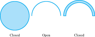
As the discussion of a clamped dot product illustrates, considering lighting equations brings up the notion of sideness to a surface. If the object is a closed surface (a sphere, for example), then it seems clear that a light shining onto the top of the sphere should not illuminate the bottom of the sphere. However, if the object is not a closed surface (a hemisphere, for example), then the exterior should be illuminated when the light source points at it, and the interior should be illuminated when the light source points inside. If the hemisphere is modeled as a single layer of polygons tiling the surface of the hemisphere, then the normal vector at each vertex can either be directed inward or outward, with the consequence that only one side of the surface is lighted regardless of the location of the light source.
Arguably, the solution to the problem is to not model objects with open surfaces, but rather to force everything to be a closed surface as in Figure 3.5. This is, in fact, the rule used by CAD programs to solve this and a number of related problems. However, since this may adversely complicate modeling for some applications, OpenGL also includes the notion of two-sided lighting. With two-sided lighting, different surface properties are used and the direction of the surface normal is flipped during the lighting computation depending on which side of a polygon is visible. To determine which side is visible, the signed area of the polygon is computed using the polygon’s window coordinates. The orientation of the polygon is give by the sign of the area computation.
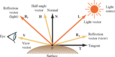
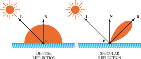
The specular term models the reflection of a light source from a smooth surface, producing a highlight focused in the direction of the reflection vector. This behavior is much different than the diffuse term, which reflects light equally in all directions, as shown in Figure 3.6. Things get a little more complicated when light isn’t equally reflected in all directions; the location of the viewer needs to be included in the equation. In the original Phong formulation, the angle between the reflection of the light vector, Rl, and viewing vector (a unit vector between the surface point and the viewer position, V) determines amount of specular reflection in the direction of the viewer.5
In the Blinn formulation used in OpenGL, however, the angle between the surface normal, and the unit bisector, H, of the light vector L, and the view vector V, is used. This bisector is also called the half-angle vector. It produces an effect similar to V · Rl, but Blinn argues that it more closely matches observed behavior, and in some circumstances is less expensive to compute.
To model surfaces of differing smoothness, this cosine term is raised to a power:
The larger this shininess exponent, n, the more polished the surface appears, and the more rapidly the contribution falls off as the reflection angle diverges from the reflection of the light vector. In OpenGL the exponent is limited to the range [0, 128], but there is least one vendor extension to allow a larger range.6
The specular term is also called the power function. OpenGL supports two different positions for the viewer: at the origin of eye space and infinitely far away along the positive z-axis. If the viewer is at infinity, (0, 0, 1)T is used for the view vector. These two viewing variations are referred to as local viewer and infinite viewer. The latter model makes the specular computation independent of the position of the surface point, thereby making it more efficient to compute. Note that this approximation is not really correct for large objects in the foreground of the scene.
To ensure that the specular contribution is zero when the surface normal is pointing away from the light source, the specular term is gated (multiplied) by a function derived from the inner product of the surface normal and light vector: fgate = (0 if N ![]() L = 0; 1 otherwise).
L = 0; 1 otherwise).
The specular term is an example of a bidirectional reflectance distribution function or BRDF–a function that is described by both the angle of incidence (the light direction) and angle of reflection (the view direction) ρ(θi, φi, θr, φr). The angles are typically defined using spherical coordinates with θ, the angle with the normal vector, and φ, the angle in the plane tangent to the normal vector. The function is also written as ρ(ωi, ωr). The BRDF represents the amount of light (in inverse steradians) that is scattered in each outgoing angle, for each incoming angle.
The emissive term models the emission of light from an object in cases where the object itself acts as a light source. An example is an object that fluoresces. In OpenGL, emission is a property of the object being shaded and does not depend on any light source. Since neither the emissive or ambient terms are dependent on the location of the light source, they don’t use a gating function the way the diffuse and specular terms do (note that the diffuse term gates itself).
3.3.1 Intensities, Colors, and Materials
So far, we have described the lighting model in terms of producing intensity values for each contribution. These intensity values are used to scale color values to produce a set of color contributions. In OpenGL, both the object and light have an RGBA color, which are multiplied together to get the final color value:

The colors associated with the object are referred to as reflectance values or reflectance coefficients. They represent the amount of light reflected (rather than absorbed or transmitted) from the surface. The set of reflectance values and the specular exponent are collectively called material properties. The color values associated with light sources are intensity values for each of the R, G, and B components. OpenGL also stores alpha component values for reflectances and intensities, though they aren’t really used in the lighting computation. They are stored largely to keep the application programming interface (API) simple and regular, and perhaps so they are available in case there’s a use for them in the future. The alpha component may seem odd, since one doesn’t normally think of objects reflecting alpha, but the alpha component of the diffuse reflectance is used as the alpha value of the final color. Here alpha is typically used to model transparency of the surface. For conciseness, the abbreviations am, dm, sm, al, dl, and sl are used to represent the ambient, diffuse, specular material reflectances and light intensities; em represents the emissive reflectance (intensity), while asc represents the scene ambient intensity.
The interaction of up to 8 different light sources with the object’s material are evaluated and combined (by summing them) to produce a final color.
3.3.2 Light Source Properties
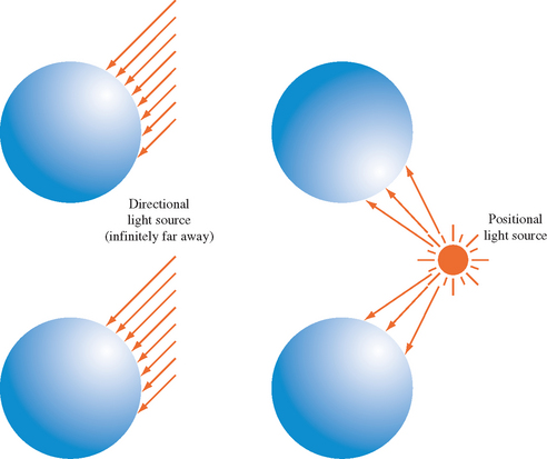
In addition to intensity values, OpenGL also defines additional properties of the light sources. Both directional (infinite lights) and positional (local lights) light sources can be emulated. The directional model simulates light sources, such as the sun, that are so distant that the lighting vector doesn’t change direction over the surface of the primitive. Since the light vector doesn’t change, directional lights are the simplest to compute. If both an infinite light source and an infinite viewer model are set, the half-angle vector used in the specular computation is constant for each light source.
Positional light sources can show two effects not seen with directional lights. The first derives from the fact that a vector drawn from each point on the surface to the light source changes as lighting is computed across the surface. This leads to changes in intensity that depend on light source position. For example, a light source located between two objects will illuminate the areas that face the light source. A directional light, on the other hand, illuminates the same regions on both objects (Figure 3.7). Positional lights also include an attenuation factor, modeling the falloff in intensity for objects that are further away from the light source:
OpenGL distinguishes between directional and positional lights with the w coordinate of the light position. If w is 0, then then the light source is at infinity, if it is non-zero then it is not. Typically, only values of 0 and 1 are used. Since the light position is transformed from object space to eye space before the lighting computation is performed (when a light position is specified), applications can easily specify the positions of light sources relative to other objects in the scene.
In addition to omnidirectional lights radiating uniformly in all directions (sometimes called point lights), OpenGL also models spotlight sources. Spotlights are light sources that have a cone-shaped radiation pattern: the illumination is brightest along the the axis of the cone, decreases from the center to the edge of the cone, and drops to zero outside the cone (as shown in Figure 3.8). This radiation pattern is parameterized by the spotlight direction (sd), cutoff angle (co), and spotlight exponent (se), controlling how rapidly the illumination falls off between the center and the edge of the cone:
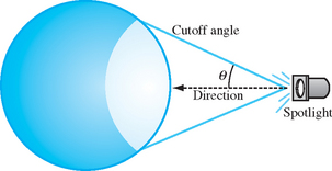
If the angle between the light vector and spot direction is greater than the cutoff angle (dot product is less than the cosine of the cutoff angle), then the spot attenuation is set to zero.
3.3.3 Material Properties
OpenGL provides great flexibility for setting material reflectance coefficients, light intensities, and other lighting mode parameters, but doesn’t specify how to choose the proper values for these parameters.
Material properties are modeled with four groups of reflectance coefficients (ambient, diffuse, specular, and emissive) and a specular exponent. In practice, the emissive term doesn’t play a significant role in modeling normal materials, so it will be ignored in this discussion.
For lighting purposes, materials can be described by the type of material, and the smoothness of its surface. Surface smoothness is simulated by the overall magnitude of the three reflectances, and the value of the specular exponent. As the magnitude of the reflectances get closer to one, and the specular exponent value increases, the material appears to have a smoother surface.
Material type is simulated by the relationship between three of the reflectances (ambient, diffuse, and specular). For classification purposes, simulated materials can be divided into four categories: dielectrics, metals, composites, and other materials.
Dielectrics This is the most common category. Dielectrics are non-conductive materials, such as plastic or wood, which don’t have free electrons. As a result, dielectrics have relatively low reflectivity; what reflectivity they do have is independent of light color. Because they don’t strongly interact with light, some dielectrics are transparent. The ambient, diffuse, and specular colors tend to have similar values in dielectric materials.
Powdered dielectrics tend to look white because of the high surface area between the powdered dielectric and the surrounding air. Because of this high surface area, they also tend to reflect diffusely.
Metals Metals are conductive and have free electrons. As a result, metals are opaque and tend to be very reflective, and their ambient, diffuse, and specular colors tend to be the same. The way free electrons react to light can be a function of the light’s wavelength, determining the color of the metal. Materials like steel and nickel have nearly the same response over all visible wavelengths, resulting in a grayish reflection. Copper and gold, on the other hand, reflect long wavelengths more strongly than short ones, giving them their reddish and yellowish colors.
The color of light reflected from metals is also a function angle between the incident or reflected light directions and the surface normal. This effect can’t be modeled accurately with the OpenGL lighting model, compromising the appearance of metallic objects. However, a modified form of environment mapping (such as the OpenGL sphere mapping) can be used to approximate the angle dependency. Additional details are described in Section 15.9.1.
Composite Materials Common composites, like plastic and paint, are composed of a dielectric binder with metal pigments suspended in them. As a result, they combine the reflective properties of metals and dielectrics. Their specular reflection is dielectric, while their diffuse reflection is like metal.
Other Materials Other materials that don’t fit into the above categories are materials such as thin films and other exotics. These materials are described further in Chapter 15.
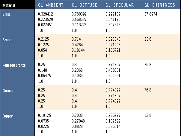
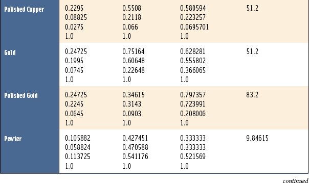
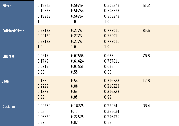
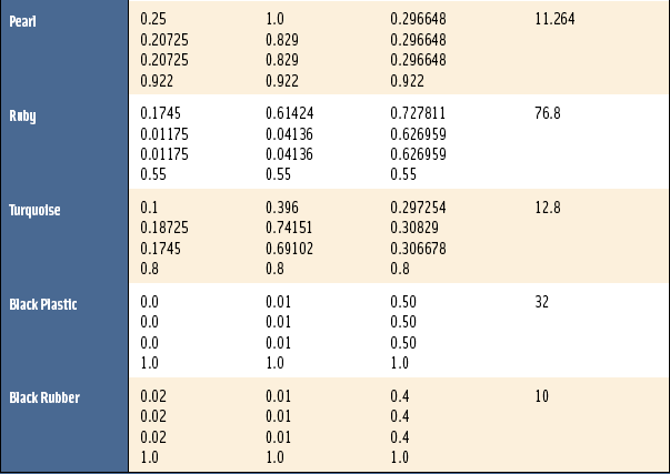
As mentioned previously, the apparent smoothness of a material is a function of how strongly it reflects and the size of the specular highlight. This is affected by the overall magnitude of the GL_AMBIENT, GL_DIFFUSE, and GL_SPECULAR parameters, and the value of GL_SHININESS. Here are some heuristics that describe useful relationships between the magnitudes of these parameters:
1. The spectral color of the ambient and diffuse reflectance parameters should be the same.
2. The magnitudes of diffuse and specular reflectance should sum to a value close to 1. This helps prevent color value overflow.
3. The value of the specular exponent should increase as the magnitude of specular reflectance approaches 1.
Using these relationships, or the values in Table 3.1, will not result in a perfect imitation of a given material. The empirical model used by OpenGL emphasizes performance, not physical exactness. Improving material accuracy requires going beyond the OpenGL lighting model to more sophisticated multipass techniques or use of the programmable pipeline. For an excellent description of material properties see Hall (1989).
3.3.4 Vertex and Fragment Lighting
Ideally the lighting model should be evaluated at each point on the object’s surface. When rendering to a framebuffer, the computation should be recalculated at each pixel. At the time the OpenGL specification was written, however, the amount of processing power required to perform these computations at each pixel was deemed too expensive to be widely available. Instead the specification uses a basic vertex lighting model.
This lighting model can provide visually appealing results with modest computation requirements, but it does suffer from a number of drawbacks. One drawback related to color representation occurs when combining lighting with texture mapping. To texture a lighted surface, the intent is to use texture samples as reflectances for the surface. This can be done by using vertex lighting to compute an intensity value at the vertex color (by setting all of the material reflectance values to 1.0) then multiplying by the reflectance value from the texture map, using the GL_MODULATE texture environment. This approach can have problems with specular surfaces, however. Only a single intensity and reflectance value can be simulated, since texturing is applied only after the lighting equation has been evaluated to a single intensity. Texture should be applied separately to compute diffuse and specular terms.
To work around this problem, OpenGL 1.2 adds a mode to the vertex lighting model, GL_SEPARATE_SPECULAR_COLOR, to generate two final color values—primary and secondary. The first color contains the sum of all of the terms except for the specular term, the second contains just the specular color. These two colors are passed into the rasterization stage, but only the primary color is modified by texturing. The secondary color is added to the primary after the texturing stage. This allows the application to use the texture as the diffuse reflectance and to use the material’s specular reflectance settings to define the object’s specular properties.
This mode and other enhancements to the lighting model are described in detail in Chapter 15.
3.4 Fixed-Point and Floating-Point Arithmetic
There is more to color representation than the number of bits per color component. Typically the transformation pipeline represents colors using some form of floating-point, often a streamlined IEEE single-precision representation. This isn’t much of a burden since the need for floating-point representation already exists for vertex, normal, and texture coordinate processing. In the transformation pipeline, RGB colors can be represented in the range [−1, 1]. The negative part of the range can be used to perform a limited amount of subtractive processing in the lighting stage, but as the colors are passed to the rasterization pipeline, toward their framebuffer destination (usually composed of unsigned integers), they are clamped to the [0, 1] range.
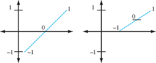
Traditionally, the rasterization pipeline uses a fixed-point representation with the requisite reduction in range and precision. The fixed-point representation requires careful implementation of arithmetic operations to avoid artifacts. The principal complexity comes from the difficulty in representing the number 1.0. A traditional fixed-point representation using 8 bits might use the most significant bit as the integer part and the remaining 7 bits as fraction. This straightforward interpretation can represent numbers in the range [0, 1.9921875], which is ![]() .
.
This representation wastes 1 bit, since it represents numbers almost up to 2, when only 1 is required. Most rasterization implementations don’t use any integer bits, instead they use a somewhat more complicated representation in which 1.0 is represented with the “all ones” bit pattern. This means that an 8-bit number x in the range [0, 1] converts to this representation using the formula f = x255. The complexity enters when implementing multiplication. For example, the identity a * 1 = a should be preserved, but the naive implementation, using a multiplication and a shift, will not do so. For example multiplying (255 * 255) and shifting right produces 254. The correct operation is (255 * 255)/255, but the expensive division operation is often replaced with a faster, but less accurate approximation.
Later revisions to OpenGL added the ability to perform subtractions at various stages of rasterization and framebuffer processing (subtractive blend7, subtractive texture environment8) using fixed-point signed values. Accurate fixed-point representation of signed values is difficult. A signed representation should preserve three identities: a * 1 = a, a * 0 = 0, and a *−1 = −a. Fixed step sizes in value should result in equal step sizes in the representation, and resolution should be maximized.
One approach is to divide the set of fixed-point values into three pieces: a 0 value, positive values increasing to 1, and negative values decreasing to negative one. Unfortunately, this can’t be done symmetrically for a representation with 2n bits. OpenGL compromises, using the representation (2n × value − 1)/2. This provides a 0, 1, and negative one value, but does so asymmetrically; there is an extra value in the negative range.
3.4.1 Biased Arithmetic
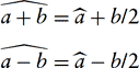
Although the accumulation buffer is the only part of the OpenGL framebuffer that directly represents negative colors, it is possible for an application to subtract color values in the framebuffer by scaling and biasing the colors and using subtractive operations. For example, numbers in the range [−1, 1] can be mapped to the [0, 1] range by scaling by 0.5 and biasing by 0.5. This effectively converts the fixed-point representation into a sign and magnitude representation.9
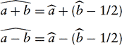
Working with biased numbers requires modifying the arithmetic rules (Figure 3.9). Assume a and b are numbers in the original representation and ![]() and
and ![]() are in the biased representation. The two representations can be converted back and forth with the following equations:
are in the biased representation. The two representations can be converted back and forth with the following equations:
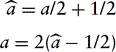
When converting between representations, the order of operations must be controlled to avoid losing information when OpenGL clamps colors to [0, 1]. For example, when converting from ![]() to a, the value of 1/2 should be subtracted first, then the result should be scaled by 2, rather than rewriting the equation as 2
to a, the value of 1/2 should be subtracted first, then the result should be scaled by 2, rather than rewriting the equation as 2![]() − 1. Biased arithmetic can be derived from these equations using substitution. Note that biased arithmetic values require special treatment before they can be operated on with regular (2′s complement) computer arithmetic; they can’t just be added and subtracted:
− 1. Biased arithmetic can be derived from these equations using substitution. Note that biased arithmetic values require special treatment before they can be operated on with regular (2′s complement) computer arithmetic; they can’t just be added and subtracted:
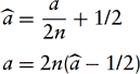
The equation ![]() is supported directly by the GL_COMBINE texture function GL_ADD_SIGNED.10
is supported directly by the GL_COMBINE texture function GL_ADD_SIGNED.10
The following equations add or subtract a regular number with a biased number, reducing the computational overhead of converting both numbers first:
This representation allows us to represent numbers in the range [−1, 1]. We can extend the technique to allow us to increase the range. For example, to represent a number in the range [−n, n], we use the equations:
and alter the arithmetic as above. The extended range need not be symmetric. We can represent a number in the range [−m, n] with the formula:
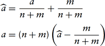
and modify the the equations for addition and subtraction as before.
With appropriate choices of scale and bias, the dynamic range can be increased, but this comes at the cost of precision. For each factor of 2 increase in range, 1 bit of precision is lost. In addition, some error is introduced when converting back and forth between representations. For an 8-bit framebuffer it isn’t really practical to go beyond [−1, 1] before losing too much precision. With higher precision framebuffers, a little more range can be obtained, but the extent to which the lost precision is tolerable depends on the application. As the rendering pipeline evolves and becomes more programmable and floating-point computation becomes pervasive in the rasterization stage of the pipeline, many of these problems will disappear. However, the expansion of OpenGL implementations to an ever-increasing set of devices means that these same problems will remain on smaller, less costly devices for some time.
3.5 Summary
This chapter provided an overview of the representation and manipulation of color values in the OpenGL pipeline. It also described some of the computational models used to shade an object, focusing on the vertex lighting model built into OpenGL. The next chapter covers some of the principles and complications involved in representing an image as an array of discrete color values.
1The term YCrCb is also used and means the same thing except the order of the two color difference signals Cb and Cr is exchanged. The name may or may not imply something about the order of the components in a pixel stream.
2More correctly, the relationship is D = (I + ∈)γ, where ∈ is a black level offset. The black level is adjusted using the brightness control on a CRT. The gamma value is adjusted using the contrast control.
3Note that when color material is enabled, the current color updates the material definition. In hindsight, it would have been cleaner and less confusing to simply use the current color in the lighting computation, but not replace the current material definition as a side effect.
4The name Phong lighting is a misnomer, the equations used in the OpenGL specification are from Blinn [Bli77].
5V · Rl can equivalently be written as L · Rv, where Rv is the reflection of the view vector V.
6NV_light_max_exponent
7In the OpenGL 1.2 ARB imaging subset.
8OpenGL 1.3.
9In traditional sign and magnitude representation, the sign bit is 1 for a negative number; in ours a sign bit of 0 represents a negative number.
10OpenGL 1.3.