Lighting Techniques
This section discusses various ways of improving and refining the lighted appearance of objects. There are several approaches to approving the fidelity of lighting. The process of computing lighting can be decomposed into separate subtasks. One is capturing the material properties of an object, reflectances, roughness, transparency, subsurface properties, and so on. A second is the direct illumination model; the manner in which the surface interacts with the light striking the target object. The third is light transport, which takes into account the overall path of light, including light passing through other mediums such as haze or water on its way to the target object. Light transport also includes indirect illumination, wherein the light source is light reflected from another surface. Computing this requires taking into account how light rays are blocked by other objects, or by parts of the target object itself, creating shadows on the target object.
Lighting is a very broad topic and continues to rapidly evolve. In this chapter we consider various algorithms for improving the quality and character of the direct illumination model and material modeling. We end by considering restricted-light-transport modeling problems, such as ambient occlusion.
15.1 Limitations in Vertex Lighting
OpenGL uses a simple per-vertex lighting facility to incorporate lighting into a scene. Section 3.3.4 discusses some of the shortcomings of per-vertex lighting. One problem is the location in the pipeline where the lighting terms are summed for each vertex. The terms are combined at the end of the vertex processing, causing problems with using texture maps as the source for diffuse reflectance properties. This problem is solved directly in OpenGL 1.2 with the addition of a separate (secondary) color for the specular term, which is summed after texturing is applied. A second solution, using a two-pass algorithm, is described in Section 9.2. This second technique is important because it represents a general class of techniques in which the terms of the vertex lighting equation are computed separately, then summed together in a different part of the pipeline.
Another problem described in Section 3.3.4 is that the lighting model is evaluated per-vertex rather than per-pixel. Per-vertex evaluation can be viewed as another form of sampling (Section 4.1); the sample points are the eye coordinates of the vertices and the functions being sampled are the various subcomponents of the lighting equation. The sampled function is partially reconstructed, or resampled, during rasterization as the vertex attributes are (linearly) interpolated across the face of a triangle, or along the length of a line.
Although per-vertex sampling locations are usually coarser than per-pixel, assuming that this results in poorer quality images is an oversimplification. The image quality depends on both the nature of the function being sampled and the set of sample points being used. If the sampled function consists of slowly varying values, it does not need as high a sample rate as a function containing rapid transitions. Reexamining the intensity terms in the OpenGL lighting equation1

shows that the ambient and emissive terms are constants and the diffuse term is fairly well behaved. The diffuse term may change rapidly, but only if the surface normal also does so, indicating that the surface geometry is itself rapidly changing. This means that per-vertex evaluation of the diffuse term doesn’t introduce much error if the underlying vertex geometry reasonably models the underlying surface. For many situations the surface can be modeled accurately enough with polygonal geometry such that diffuse lighting gives acceptable results. An interesting set of surfaces for which the results are not acceptable is described in Sections 15.9.3 and 15.10.
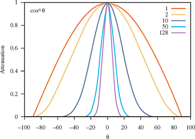
Accurate specular component sampling becomes more challenging to sample when the specular exponent (shininess) is greater than 1. The specular function—a cosine power function-varies rapidly when evaluated with large exponents. Small changes in the surface normal results in large changes in the specular contribution. Figure 15.1 shows the result of exponentiating the cosine function for several different exponent values. This, of course, is the desired effect for the specular term. It models the rapid fall-off of a highlight reflected from a polished surface. This means that shiny surfaces must be modeled with greater geometric accuracy to correctly capture the specular contribution.
15.1.1 Static and Adaptive Tessellation
We’ve seen that highly specular surfaces need to be modeled more accurately than diffuse surfaces. We can use this information to generate better models. Knowing the intended shininess of the surface, the surface can be tessellated until the difference between (H · N)n at triangle vertices drops below a predetermined threshold. An advantage of this technique is that it can be performed during modeling; perferably as a preprocessing step as models are converted from a higher-order representation to a polygonal representation. There are performance versus quality trade-offs that should also be considered when deciding the threshold. For example, increasing the complexity (number of triangles) of a modeled object may substantially affect the rendering performance if:
• The performance of the application or system is already vertex limited: geometry processing, rather than fragment processing, limits performance.
• The model has to be clipped against a large number of application-defined clipping planes.
The previous scheme statically tessellates each object to meet quality requirements. However, because the specular reflection is view dependent only a portion of the object needs to be tessellated to meet the specular quality requirement. This suggests a scheme in which each model in the scene is adaptively tessellated. Then only parts of each surface need to be tessellated. The difficulty with such an approach is that the cost of retessellating each object can be prohibitively expensive to recompute each frame. This is especially true if we also want to avoid introducing motion artifacts caused by adding or removing object vertices between frames.
For some specific types of surfaces, however, it may be practical to build this idea into the modeling step and generate the correct model at runtime. This technique is very similar to the geometric level of detail techniques described in Section 16.4. The difference is that model selection uses specular lighting (see Figure 15.2) accuracy as the selection criterion, rather than traditional geometric criteria such as individual details or silhouette edges.

15.1.2 Local Light and Spotlight Attenuation
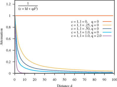
Like specular reflection, a vertex sampling problem occurs when using distance-based and spotlight attenuation terms. With distance attenuation, the attenuation function is not well behaved because it contains reciprocal terms:
Figure 15.3 plots values of the attenuation function for various coefficients. When the linear or quadratic coefficients are non-zero, the function tails off very rapidly. This means that very fine model tessellation is necessary near the regions of rapid change, in order to capture the changes accurately.
With spotlights, there are two sources of problems. The first comes from the cutoff angle defined in the spotlight equation. It defines an abrupt cutoff angle that creates a discontinuity at the edge of the cone. Second, inside the cone a specular-like power function is used to control intensity drop-off:
When the geometry undersamples the lighting model, it typically manifests itself as a dull appearance across the illuminated area (cone), or irregular or poorly defined edges at the perimeter of the illuminated area. Unlike the specular term, the local light and spotlight attenuation terms are a property of the light source rather than the object. This means that solutions involving object modeling or tessellation require knowing which objects will be illuminated by a particular light source. Even then, the sharp cutoff angle of a spotlight requires tessellation nearly to pixel-level detail to accurately sample the cutoff transition.
15.2 Fragment Lighting Using Texture Mapping
The preceding discussion and Section 3.3.4 advocate evaluating lighting equations at each fragment rather than at each vertex. Using the ideas from the multipass toolbox discussed in Section 9.3, we can efficiently approximate a level of per-fragment lighting computations using a combination of texture mapping and framebuffer blending. If multitexture, the combine texture environment, and vertex and fragment program features are available,2 we can implement these algorithms more efficiently or use more sophisticated ones. We’ll start by presenting the general idea, and then look at some specific techniques.
Abstractly, the texture-mapping operation may be thought of as a function evaluation mechanism using lookup tables. Using texture mapping, the texture-matrix and texture-coordinate generation functions can be combined to create several useful mapping algorithms. The first algorithm is a straightforward 1D and 2D mapping of f(s) and f(s, t). The next is the projective mappings described in Section 14.9: f(s, t, r, q). The third uses environment and reflection mapping techniques with sphere and cube maps to evaluate f(R).
Each mapping category can evaluate a class of equations that model some form of lighting. Taking advantage of the fact that lighting contributions are additive-and using the regular associative, commutative, and distributive properties of the underlying color arithmetic-we can use framebuffer blending in one of two ways. It can be used to sum partial results or to scale individual terms. This means that we can use texture mapping and blending as a set of building blocks for computing lighting equations. First, we will apply this idea to the problematic parts of the OpenGL lighting equation: specular highlights and attenuation terms. Then we will use the same ideas to evaluate some variations on the standard (traditional) lighting models.
15.3 Spotlight Effects Using Projective Textures
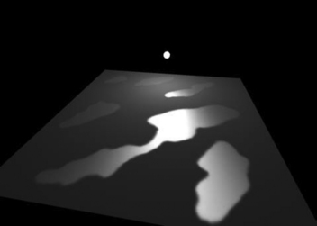
The projective texture technique (described in Section 14.9) can be used to generate a number of interesting illumination effects. One of them is spotlight illumination. The OpenGL spotlight illumination model provides control over a cutoff angle (the spread of the light cone), an intensity exponent (concentration across the cone), the direction of the spotlight, and intensity attenuation as a function of distance. The core idea is to project a texture map from the same position as the light source that acts as an illumination mask, attenuating the light source. The mask is combined with a point light source placed at the spotlight’s position. The texture map captures the cutoff angle and exponent, whereas the vertex light provides the rest of the diffuse and specular computation. Because the projective method samples the illumination at each pixel, the undersampling problem is greatly reduced.
The texture is an intensity map of a cross section of the spotlight’s beam. The same exponent parameters used in the OpenGL model can be incorporated, or an entirely different model can be used. If 3D textures are available, attenuation due to distance can also be approximated using a texture in which the intensity of the cross section is attenuated along the r dimension. As geometry is rendered with the spotlight projection, the r coordinate of the fragment is proportional to the distance from the light source.
To determine the transformation needed for the texture coordinates, it helps to consider the simplest case: the eye and light source are coincident. For this case, the texture coordinates correspond to the eye coordinates of the geometry being drawn. The coordinates could be explicitly computed by the application and sent to the pipeline, but a more efficient method is to use an eye-linear texture generation function.
The planes correspond to the vertex coordinate planes (e.g., the s coordinate is the distance of the vertex coordinate from the y-z plane, and so on). Since eye coordinates are in the range [-1.0, 1.0] and the texture coordinates need to be in the range [0.0, 1.0], a scale and bias of 0.5 is applied to s and t using the texture matrix. A perspective spotlight projection transformation can be computed using gluPerspective and combined into the texture transformation matrix.
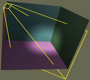
The transformation for the general case, when the eye and light source are not in the same position, can be computed by compositing an additional transform into the texture matrix. To find the texture transform for a light at an arbitrary location, the new transform should be the inverse of the transformations needed to move the light source from the eye position to the location. Once the texture map has been created, the method for rendering the scene with the spotlight illumination (see Figure 15.4) is:
1. Initialize the depth buffer.
2. Clear the color buffer to a constant value representing the scene ambient illumination.
3. Drawing the scene with depth buffering enabled and color buffer writes disabled (pass 1).
4. Load and enable the spotlight texture, and set the texture environment to GL_MODULATE.
5. Enable the texture generation functions, and load the texture matrix.
6. Enable blending and set the blend function to GL_ONE, GL_ONE.
7. Disable depth buffer updates and set the depth function to GL_EQUAL.
8. Draw the scene with the vertex colors set to the spotlight color (pass 2).
9. Disable the spotlight texture, texgen, and texture transformation.
10. Set the blend function to GL_DST_COLOR.
11. Draw the scene with normal diffuse and specular illumination (pass 3).
There are three passes in the algorithm. At the end of the first pass the ambient illumination has been established in the color buffer and the depth buffer contains the resolved depth values for the scene. In the second pass, the illumination from the spotlight is accumulated in the color buffer. By using the GL_EQUAL depth function, only visible surfaces contribute to the accumulated illumination. In the final pass the scene is drawn with the colors modulated by the illumination accumulated in the first two passes to compute the final illumination values.
The algorithm does not restrict the use of texture on objects, because the spotlight texture is only used in the second pass; only the scene geometry is needed in this one. The second pass can be repeated multiple times with different spotlight textures and projections to accumulate the contributions of multiple spotlight sources.
There are some caveats to consider when implementing this technique. Texture projection along the negative line-of-sight of the texture (back projection) can contribute undesired illumination to the scene. This can be eliminated by positioning a clip plane at the near plane of the projection line-of-site. The clip plane is enabled during the spotlight illumination pass, and oriented to remove objects rendered behind the spotlight.
OpenGL encourages but does not guarantee invariance when arbitrary modes are enabled or disabled. This can manifest itself in undesirable ways during multipass algorithms. For example, enabling texture coordinate generation may cause fragments with different depth values to be generated compared to the one generated when texture coordinate generation is not enabled. This problem can be overcome by reestablishing the depth buffer values between the second and third pass. Do this by redrawing the scene with color buffer updates disabled and depth buffering configured as it was during the first pass.
Using a texture wrap mode of GL_CLAMP will keep the spotlight pattern from repeating. When using a linear texture filter, use a black texel border to avoid clamping artifacts; or, if available, use the GL_CLAMP_TO_EDGE wrap mode.3
15.4 Specular Lighting Using Environment Maps
The appearance of the OpenGL per-vertex specular highlight can be improved by using environment mapping to generate a higher-quality per-pixel highlight. A sphere map containing only a Phong highlight (Phong, 1975) is applied to the object and the result is summed with the object’s per-vertex ambient and diffuse lighting contributions to create the final, lighted color (see Figure 15.5). The environment map uses the eye reflection vector, Rv, to index the texture map, and thus it can be used like a lookup table to compute the specular term:
For each polygon in the object, the reflection vector is computed at each vertex. This technique interpolates the sphere-mapped coordinates of the reflection vector instead of the highlight itself, and thus a much more accurate sampling of the highlight is achieved. The sphere map image for the texture map of the highlight is computed by rendering a highly tessellated sphere, lighted with a specular highlight. Using the OpenGL pipeline to compute the specular color produces a Blinn (rather than Phong) specular function. If another function is required, the application can evaluate the specular function at each vertex and send the result to the pipeline as a vertex color. The bidirectional function, f(L, R), is reduced to a function of a single direction by encoding the direction of the light (L) relative to the view direction into the texture map. Consequently, the texture map needs to be recomputed whenever the light or viewer position is changed. Sphere mapping assumes that the view direction is constant (infinite viewer) and the environment (light) direction is infinitely far away. As a result, the highlight does not need to be changed when the object moves. Assuming a texture map is also used to provide the object’s diffuse reflectance, the steps in the two-pass method are:
1. Define the material with appropriate diffuse and ambient reflectance, and zero for the specular reflectance coefficients.
3. Define and enable texture to be combined with diffuse lighting.
4. Define modulate texture environment.
5. Draw the lighted, textured object into the color buffer.
7. Load the sphere map texture, and enable the sphere map texgen function.
8. Enable blending, and set the blend function to GL_ONE, GL_ONE.
9. Draw the unlighted, textured geometry with vertex colors set to the specular material color.
15.4.1 Multitexture
If a texture isn’t used for the diffuse color, then the algorithm reduces to a single pass using the add texture environment (see Figure 15.5) to sum the colors rather than framebuffer blending. For this technique to work properly, the specular material color should be included in the specular texture map rather than in the vertex colors. Multiple texture units can also be used to reduce the operation to a single pass. For two texture units, the steps are modified as follows:
1. Define the material with appropriate diffuse and ambient reflectance, and zero for the specular reflectance coefficients.
3. Define and enable texture to be combined with diffuse lighting in unit 0.
4. Set modulate texture environment for unit 0.
5. Load the sphere map texture, and enable the sphere map texgen function for unit 1.
As with the separate specular color algorithm, this algorithm requires that the specular material reflectance be premultiplied with the specular light color in the specular texture map.
With a little work the technique can be extended to handle multiple light sources. The idea can be further generalized to include other lighting models. For example, a more accurate specular function could be used rather than the Phong or Blinn specular terms. It can also include the diffuse term. The algorithm for computing the texture map must be modified to encompass the new lighting model. It may still be useful to generate the map by rendering a finely tessellated sphere and evaluating the lighting model at each vertex within the application, as described previously. Similarly, the technique isn’t restricted to sphere mapping; cube mapping, dual-paraboloid mapping, and other environment or normal mapping formulations can be used to yield even better results.
15.5 Light Maps
A light map is a texture map applied to an object to simulate the distance-related attenuation of a local light source. More generally, light maps may be used to create nonisotropic illumination patterns. Like specular highlight textures, light maps can improve the appearance of local light sources without resorting to excessive tessellation of the objects in the scene. An excellent example of an application that uses light maps is the Quake series of interactive PC games (id Software, 1999). These games use light maps to simulate the effects of local light sources, both stationary and moving, to great effect.
There are two parts to using light maps: creating a texture map that simulates the light’s effect on an object and specifying the appropriate texture coordinates to position and shape the light. Animating texture coordinates allows the light source (or object) to move. A texture map is created that simulates the light’s effect on some canonical object. The texture is then applied to one or more objects in the scene. Appropriate texture coordinates are applied using either object modeling or texture coordinate generation. Texture coordinate transformations may be used to position the light and to create moving or changing light effects. Multiple light sources can be generated with a combination of more complex texture maps and/or more passes to the algorithm.
Light maps are often luminance (single-component) textures applied to the object using a modulate texture environment function. Colored lights are simulated using an RGB texture. If texturing is already used for the material properties of an object, either a second texture unit or a multipass algorithm is needed to apply the light map. Light maps often produce satisfactory lighting effects using lower resolution than that normally needed for surface textures. The low spatial resolution of the texture usually does not require mipmapping; choosing GL_LINEAR for the minification and magnification filters is sufficient. Of course, the quality requirements for the lighting effect are dependent on the application.
15.5.1 2D Texture Light Maps
A 2D light map is a 2D luminance map that modulates the intensity of surfaces within a scene. For an object and a light source at fixed positions in the scene, a luminance map can be calculated that exactly matches a surface of the object. However, this implies that a specific texture is computed for each surface in the scene. A more useful approximation takes advantage of symmetry in isotropic light sources, by building one or more canonical projections of the light source onto a surface. Translate and scale transformations applied to the texture coordinates then model some of the effects of distance between the object and the light source. The 2D light map may be generated analytically using a 2D quadratic attenuation function, such as
This can be generated using OpenGL vertex lighting by drawing a high-resolution mesh with a local light source positioned in front of the center of the mesh. Alternatively, empirically derived illumination patterns may be used. For example, irregularly shaped maps can be used to simulate patterns cast by flickering torches, explosions, and so on.
A quadratic function of two inputs models the attenuation for a light source at a fixed perpendicular distance from the surface. To approximate the effect of varying perpendicular distance, the texture map may be scaled to change the shape of the map. The scaling factors may be chosen empirically, for example, by generating test maps for different perpendicular distances and evaluating different scaling factors to find the closest match to each test map. The scale factor can also be used to control the overall brightness of the light source. An ambient term can also be included in a light map by adding a constant to each texel value. The ambient map can be a separate map, or in some cases combined with a diffuse map. In the latter case, care must be taken when applying maps from multiple sources to a single surface.
To apply a light map to a surface, the position of the light in the scene must be projected onto each surface of interest. This position determines the center of the projected map and is used to compute the texture coordinates. The perpendicular distance of the light from the surface determines the scale factor. One approach is to use linear texture coordinate generation, orienting the generating planes with each surface of interest and then translating and scaling the texture matrix to position the light on the surface. This process is repeated for every surface affected by the light.
To repeat this process for multiple lights (without resorting to a composite multilight light map) or to light textured surfaces, the lighting is done using multiple texture units or as a series of rendering passes. In effect, we are evaluating the equation
The difficulty is that the texture coordinates used to index each of the light maps (I1, …, In) are different because the light positions are different. This is not a problem, however, because multiple texture units have independent texture coordinates and coordinate generation and transformation units, making the algorithm using multiple texture units straightforward. Each light map is loaded in a separate texture unit, which is set to use the add environment function (except for the first unit, which uses replace). An additional texture unit at the end of the pipeline is used to store the surface detail texture. The environment function for this unit is set to modulate, modulating the result of summing the other textures. This rearranges the equation to
where Cobject is stored in a texture unit. The original fragment colors (vertex colors) are not used. If a particular object does not use a surface texture, the environment function for the last unit (the one previously storing the surface texture) is changed to the combine environment function with the GL_SOURCE0_RGB and GL_SOURCE0_ALPHA parameters set to GL_PRIMARY_COLOR. This changes the last texture unit to modulate the sum by the fragment color rather than the texture color (the texture color is ignored).
If there aren’t enough texture units available to implement a multitexture algorithm, there are several ways to create a multipass algorithm instead. If two texture units are available, the units can be used to hold a light map and the surface texture. In each pass, the surface texture is modulated by a different light map and the results summed in the framebuffer. Framebuffer blending with GL_ONE as the source and destination blend factors computes this sum. To ensure visible surfaces in later passes aren’t discarded, use GL_LEQUAL for the depth test. In the simple case, where the object doesn’t have a surface texture, only a single texture unit is needed to modulate the fragment color.
If only a single texture unit is available, an approximation can be used. Rather than computing the sum of the light maps, compute the product of the light maps and the object.
This allows all of the products to be computed using framebuffer blending with source and destination factors GL_ZERO and GL_SRC_COLOR. Because the multiple products rapidly attenuate the image luminance, the light maps are pre-biased or brightened to compensate. For example, a biased light map might have its range transformed from [0.0, 1.0] to [0.5, 1.0]. An alternative, but much slower, algorithm is to have a separate color buffer to compute each CobjectIj term using framebuffer blending, and then adding this separate color buffer onto the scene color buffer. The separate color buffer can be added by using glCopyPixels and the appropriate blend function. The visible surfaces for the object must be correctly resolved before the scene accumulation can be done. The simplest way to do this is to draw the entire scene once with color buffer updates disabled. Here is summary of the steps to support 2D light maps without multitexture functionality:
1. Create the 2D light maps. Avoid artifacts by ensuring the intensity of the light map is the same at all edges of the texture.
2. Define a 2D texture, using GL_REPEAT for the wrap values in s and t. Minification and magnification should be GL_LINEAR to make the changes in intensity smoother.
3. Render the scene without the light map, using surface textures as appropriate.
4. For each light in the scene, perform the following. For each surface in the scene:
(a) Cull the surface if it cannot “see” the current light.
(b) Find the plane of the surface.
(c) Align the GL_EYE_PLANE for GL_S, and GL_T with the surface plane.
(d) Scale and translate the texture coordinates to position and size the light on the surface.
(e) Render the surface using the appropriate blend function and light map texture.
If multitexture is available, and assuming that the number of light sources is less than the number of available texture units, the set of steps for each surface reduces to:
(a) Determine set of lights affecting surface; cull surface if none.
(b) Bind the corresponding texture maps.
(c) Find the plane of the surface.
(d) For each light map, align the GL_EYE_PLANE for GL_S and GL_T with the surface plane.
(e) For each light map, scale and translate the texture coordinates to position and size the light on the surface.
(f) Set the texture environment to sum the light map contributions and modulate the surface color (texture) with that sum.
15.5.2 3D Texture Light Maps
3D textures may also be used as light maps. One or more light sources are represented as 3D luminance data, captured in a 3D texture and then applied to the entire scene. The main advantage of using 3D textures for light maps is that it is simpler to approximate a 3D function, such as intensity as a function of distance. This simplifies calculation of texture coordinates. 3D texture coordinates allow the textured light source to be positioned globally in the scene using texture coordinate transformations. The relationship between light map texture and lighted surfaces doesn’t have to be specially computed to apply texture to each surface; texture coordinate generation (glTexGen) computes the proper s, t, and r coordinates based on the light position.
As described for 2D light maps, a useful approach is to define a canonical light volume as 3D texture data, and then reuse it to represent multiple lights at different positions and sizes. Texture translations and scales are applied to shift and resize the light. A moving light source is created by changing the texture matrix. Multiple lights are simulated by accumulating the results of each light source on the scene. To avoid wrapping artifacts at the edge of the texture, the wrap modes should be set to GL_CLAMP for s, t, and r and the intensity values at the edge of the volume should be equal to the ambient intensity of the light source.
Although uncommon, some lighting effects are difficult to render without 3D textures. A complex light source, whose brightness pattern is asymmetric across all three major axes, is a good candidate for a 3D texture. An example is a “glitter ball” effect in which the light source has beams emanating out from the center, with some beams brighter than others, and spaced in a irregular pattern. A complex 3D light source can also be combined with volume visualization techniques, allowing fog or haze to be added to the lighting effects. A summary of the steps for using a 3D light map follows.
1. Create the 3D light map. Avoid artifacts by ensuring the intensity of the light map is the same at all edges of the texture volume.
2. Define a 3D texture, using GL_REPEAT for the wrap values in s, t, and r. Minification and magnification should be GL_LINEAR to make the changes in intensity smoother.
3. Render the scene without the light map, using surface textures as appropriate.
4. Define planes in eye space so that glTexGen will cause the texture to span the visible scene.
5. If the lighted surfaces are textured, adding a light map becomes a multitexture or multipass technique. Use the appropriate environment or blending function to modulate the surface color.
6. Render the image with the light map, and texgen enabled. Use the appropriate texture transform to position and scale the light source correctly.
With caveats similar to those for 2D light maps, multiple 3D light maps can be applied to a scene and mixed with 2D light maps.
Although 3D light maps are more expressive, there are some drawbacks too. 3D textures are often not well accelerated in OpenGL implementation, so applications may suffer serious reductions in performance. Older implementations may not even support 3D textures, limiting portability. Larger 3D textures use substantial texture memory resources. If the texture map has symmetry it may be exploited using a mirrored repeat texture wrap mode.4 This can reduce the amount of memory required by one-half per mirrored dimension. In general, though, 2D textures make more efficient light maps.
15.6 BRDF-based Lighting
The methods described thus far have relied largely on texture mapping to perform table lookup operations of a precomputed lighting environment, applying them at each fragment. The specular environment mapping technique can be generalized to include other bidirectional reflectance distribution functions (BRDFs), with any form of environment map (sphere, cube, dual-paraboloid). However, the specular scheme only works with a single input vector, whereas BRDFs are a function of two input vectors (L and R), or in spherical coordinates a function of four scalars f(,θi, φi, θr, φr). The specular technique fixes the viewer and light positions so that as the object moves only the reflection vector varies.
Another approach decomposes or factors the 4D BRDF function into separate functions of lower dimensionality and evaluates them separately. Each factor is stored in a separate texture map and a multipass or multitexture algorithm is used to linearly combine the components (Kautz, 1999; McCool, 2001). While a detailed description of the factorization algorithm is beyond the scope of this book, we introduce the idea because the method described by McCool et al. (McCool, 2001) allows a BRDF to be decomposed to two 2D environment maps and recombined using framebuffer (or accumulation buffer) blending with a small number of passes.
15.7 Reflectance Maps
The techniques covered so far have provided alternative methods to represent light source information or the diffuse and ambient material reflectances for an object. These methods allow better sampling without resorting to subdividing geometry. These benefits can be extended to other applications by generalizing lighting techniques to include other material reflectance parameters.
15.7.1 Gloss Maps
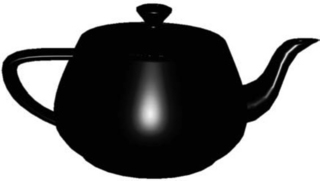
Surfaces whose shininess varies-such as marble, paper with wet spots, or fabrics that are smoothed only in places-can be modeled with gloss maps. A gloss map is a texture map that encodes a mask of the specular reflectance of the object. It modulates the result of the specular lighting computation, but is ignored in the diffues and other terms of the lighting computation (see Figure 15.6).
This technique can be implemented using a two-pass multipass technique. The diffuse, ambient, and emissive lighting components are drawn, and then the specular lighting component is added using blending.
In the first pass, the surface is drawn with ambient and diffuse lighting, but no specular lighting. This can be accomplished by setting the specular material reflectance to zero. In the second pass, the surface is drawn with the specular color restored and the diffuse, ambient, and emissive colors set to zero. The surface is textured with a texture map encoding the specular reflectance (gloss). The texture can be a one-component alpha texture or a two- or four-component texture with luminance or color components set to one.
Typically the alpha component stores the gloss map value directly, with zero indicating no specular reflection and one indicating full specular reflection. The second pass modulates the specular color-computed using vertex lighting, with the alpha value from the texture map-and sums the result in the framebuffer. The source and destination blend factors GL_SRC_ALPHA and GL_ONE perform both the modulation and the sum. The second pass must use the standard methods to allow drawing the same surface more than once, using either GL_EQUAL for the depth function or stenciling (Section 9.2).
The net result is that we compute one product per pass of Cfinal = MdId + MsIs, where Mi is the material reflectance, stored as a texture, and Ij is the reflected light intensity computed using vertex lighting. Trying to express this as single-pass multitexture algorithm with the cascade-style environment combination doesn’t really work. The separate specular color is only available post-texture, and computing the two products and two sums using texture maps for Md and Ms really requires a multiply-add function to compute a product and add the previous sum in a single texture unit. This functionality is available in vendor-specific extensions. However, using an additional texture map to compute the specular highlight (as described in Section 15.4) combined with a fragment program provides a straightforward solution. The first texture unit stores Md and computes the first product using the result of vertex lighting. The alpha component of Md also stores the gloss map (assuming it isn’t needed for transparency). The second texture unit stores the specular environment map and the two products are computed and summed in the fragment program.
15.7.2 Emission Maps
Surfaces that contain holes, windows, or cracks that emit light can be modeled using emission maps. Emission maps are similar to the gloss maps described previously, but supply the emissive component of the lighting equation rather than the specular part. Since the emissive component is little more than a pass-through color, the algorithm for rendering an emission map is simple. The emission map is an RGBA texture; the RGB values represent the emissive color, whereas the alpha values indicate where the emissive color is present. The emissive component is accumulated in a separate drawing pass for the object using a replace environment function and GL_SRC_ALPHA and GL_ONE for the source and destination blend factors. The technique can easily be combined with the two-pass gloss map algorithm to render separate diffuse, specular, and emissive contributions.
15.8 Per-fragment Lighting Computations
Rather than relying entirely on texture mapping as a simple lookup table for supplying precomputed components of the lighting equation, we can also use multitexture environments and fragment programs to directly evaluate parts of the lighting model. OpenGL 1.3 adds the combine environment and the DOT3 combine function, along with cube mapping and multitexture. These form a powerful combination for computing per-fragment values useful in lighting equations, such as N-L. Fragment programs provide the capability to perform multiple texture reads and arithmetic instructions enabling complex equations to be evaluated at each fragment. These instructions include trignometric, exponential, and logarithmic functions-virtually everything required for evaluating many lighting models.
One of the challenges in evaluating lighting at each fragment is computing the correct values for various vector quantities (for example, the light, half-angle, and normal vectors). Some vector quantities we can interpolate across the face of a polygon. We can use the cube mapping hardware to renormalize a vector (described in Section 15.11.1).
Sometimes it can be less expensive to perform the computation in a different coordinate system, transforming the input data into these coordinates. One example is performing computations in tangent space. A surface point can be defined by three perpendicular vectors: the surface normal, tangent, and binormal. The binormal and tangent vector form a plane that is tangent to the surface point. In tangent space, the surface normal is aligned with the z axis and allows a compact representation. Lighting computations are performed in tangent space by transforming (rotating) the view and light vectors. Transforming these vectors into tangent space during vertex processing can make the per-fragment lighting computations substantially simpler and improve performance. Tangent space computations and the transformation into tangent space are described in more detail in Section 15.10.2.
15.9 Other Lighting Models
Up to this point we have largely discussed the Blinn lighting model. The diffuse and specular terms for a single light are given by the following equation.
Section 15.4 discusses the use of sphere mapping to replace the OpenGL per-vertex specular illumination computation with one performed per-pixel. The specular contribution in the texture map is computed using the Blinn formulation given previously. However, the Blinn model can be substituted with other bidirectional reflectance distribution functions to achieve other lighting effects. Since the texture coordinates are computed using an environment mapping function, the resulting texture mapping operation accurately approximates view-dependent (specular) reflectance distributions.
15.9.1 Fresnel Reflection
A useful enhancement to the lighting model is to add a Fresnel reflection term, Fλ (Hall, 1989), to the specular equation:
The Fresnel term specifies the ratio of the amount of reflected light to the amount of transmitted (refracted) light. It is a function of the angle of incidence (θi), the relative index of refraction (nλ) and the material properties of the object (dielectric, metal, and so on, as described in Section 3.3.3).
Here, θ is the angle between V and the halfway vector H (cos θ = H · V). The effect of the Fresnel term is to attenuate light as a function of its incident and reflected directions as well as its wavelength. Dielectrics (such as glass) barely reflect light at normal incidence, but almost totally reflect it at glancing angles. This attenuation is independent of wavelength. The absorption of metals, on the other hand, can be a function of the wavelength. Copper and gold are good examples of metals that display this property. At glancing angles, the reflected light color is unaltered, but at normal incidence the light is modulated by the color of the metal.
Since the environment map serves as a table indexed by the reflection vector, the Fresnel effects can be included in the map by simply computing the specular equation with the Fresnel term to modulate and shift the color. This can be performed as a postprocessing step on an existing environment map by computing the Fresnel reflection coefficient at each angle of incidence and modulating the sphere or cube map. Environment mapping, reflection, and refraction and are discussed in more detail in Sections 5.4 and 17.1.
Alternatively, for direct implementation in a fragment program an approximating function can be evaluated in place of the exact Fresnel term. For example, Schlick proposes the function (Schlick, 1992)
where Cλ = (n1 − n2)2/(n1 + n2)2 and n1 is the index of refraction of the medium the incident ray passes through (typically air) and n2 the index of refraction of the material reflecting the light. Other proposed approximations are:
15.9.2 Gaussian Reflection
The Phong lighting equation, with its cosine raised to a power term for the specular component, is a poor fit to a physically accurate specular reflectance model. It’s difficult to map measured physical lighting properties to its coefficient, and at low specularity it doesn’t conserve incident and reflected energy. The Gaussian BRDF is a better model, and with some simplifications can be approximated by modifying parameters in the Phong model. The specular Phong term Kscos(θ)spec is augmented by modifying the Ks and spec parameters to a more complex and physically accurate form:  , where α is a material parameter. See Diefenbach (1997) or Ward (1992) for details on this equation’s derivation, limits to its accuracy, and material properties modeled by the α parameter. This model can be implemented either using the specular environment mapping technique described in Section 15.4 or using a fragment program.
15.9.3 Anisotropic Lighting
Traditional lighting models approximate a surface as having microscopic facets that are uniformly distributed in any direction on the surface. This uniform distribution of facets serves to randomize the direction of reflected light, giving rise to the familiar isotropic lighting behavior.
Some surfaces have a directional grain, made from facets that are formed with a directional bias, like the grooves formed by sanding or machining. These surfaces demonstrate anisotropic lighting properties, which depend on the rotation of the surface around its normal. At normal distances, the viewer does not see the facets or grooves, but only the resulting lighting effect. Some everyday surfaces that have anisotropic lighting behavior are hair, satin Christmas tree ornaments, brushed alloy wheels, CDs, cymbals in a drum kit, and vinyl records.
Heidrich and Seidel (Heidrich 1998a) present a technique for rendering surfaces with anisotropic lighting, based on the scientific visualization work of Zöckler et al. (Zöckler, 1997). The technique uses 2D texturing to provide a lighting solution based on a “most significant” normal to a surface at a point.
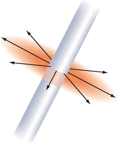
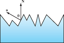
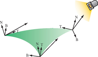
The algorithm uses a surface model with infinitely thin fibers running across the surface. The tangent vector T, defined at each vertex, can be thought of as the direction of a fiber. An infinitely thin fiber can be considered to have an infinite number of surface normals distributed in the plane perpendicular to T, as shown in Figure 15.7. To evaluate the lighting model, one of these candidate normal vectors must be chosen for use in the lighting computation.
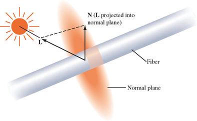
As described in Stalling (1997), the normal vector that is coplanar to the tangent vector T and light vector L is chosen. This vector is the projection of the light vector onto the normal plane as shown in Figure 15.8.
The diffuse and specular lighting factors for a point based on the view vector V, normal N, light reflection vector Rl, light direction L, and shininess exponent s are:
To avoid calculating N and Rl, the following substitutions allow the lighting calculation at a point on a fiber to be evaluated with only L, V, and the fiber tangent T (anisotropic bias).
If V and L are stored in the first two rows of a transformation matrix, and T is transformed by this matrix, the result is a vector containing L · T and V · T. After applying this transformation, L · T is computed as texture coordinate s and V · T is computed as t, as shown in Equation 15.1. A scale and bias must also be included in the matrix in order to bring the dot product range [-1, 1] into the range [0, 1]. The resulting texture coordinates are used to index a texture storing the precomputed lighting equation.
If the following simplifications are made-the viewing vector is constant (infinitely far away) and the light direction is constant-the results of this transformation can be used to index a 2D texture to evaluate the lighting equation based solely on providing T at each vertex.
The application will need to create a texture containing the results of the lighting equation (for example, the OpenGL model summarized in Appendix B.7). The s and t coordinates must be scaled and biased back to the range [-1, 1], and evaluated in the previous equations to compute N · L and V · Rl.
A transformation pipeline typically transforms surface normals into eye space by premultiplying by the inverse transpose of the viewing matrix. If the tangent vector (T) is defined in model space, it is necessary to query or precompute the current modeling transformation and concatenate the inverse transpose of that transformation with the transformation matrix in Equation 15.1.
The transformation is stored in the texture matrix and T is issued as a per-vertex texture coordinate. Unfortunately, there is no normalization step in the OpenGL texture coordinate generation system. Therefore, if the modeling matrix is concatenated as mentioned previously, the texture coordinates representing vectors may be transformed so that they are no longer unit length. To avoid this, the coordinates must be transformed and normalized by the application before transmission.
Since the anisotropic lighting approximation given does not take the self-occluding effect of the parts of the surface facing away from the light, the texture color needs to be modulated with the color from a saturated per-vertex directional light. This clamps the lighting contributions to zero on parts of the surface facing away from the illumination source.
This technique uses per-vertex texture coordinates to encode the anisotropic direction, so it also suffers from the same sampling-related per-vertex lighting artifacts found in the isotropic lighting model. If a local lighting or viewing model is desired, the application must calculate L or V, compute the entire anisotropic lighting contribution, and apply it as a vertex color.
Because a single texture provides all the lighting components up front, changing any of the colors used in the lighting model requires recalculating the texture. If two textures are used, either in a system with multiple texture units or with multipass, the diffuse and specular components may be separated and stored in two textures. Either texture may be modulated by the material or vertex color to alter the diffuse or specular base color separately without altering the maps. This can be used, for example, in a database containing a precomputed radiosity solution stored in the per-vertex color. In this way, the diffuse color can still depend on the orientation of the viewpoint relative to the tangent vector but only changes within the maximum color calculated by the radiosity solution.
15.9.4 Oren-Nayar Model
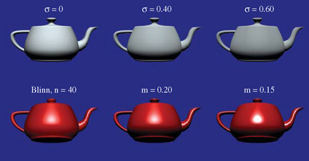
The Lambertian diffuse model assumes that light reflected from a rough surface is dependent only on the surface normal and light direction, and therefore a Lambertian surface is equally bright in all directions. This model conflicts with the observed behavior for diffuse surfaces such as the moon. In nature, as surface roughness increases the object appears flatter; the Lambertian model doesn’t capture this characteristic.
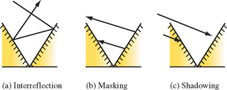
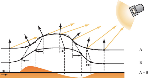
In 1994, Oren and Nayar (Oren, 1994) derived a physically-based model and validated it by comparing the results of computations with measurements on real objects. In this model, a diffuse surface is modeled as a collection of “V-cavities” as proposed by Torrance and Sparrow (Torrance, 1976). These cavities consist of two long, narrow planar facets where each facet is modeled as a Lambertian reflector. Figure 15.9 illustrates a cross-section of a surface modeled as V-cavities. The collection of cavity facets exhibit complex interactions, including interreflection, masking of reflected light, and shadowing of other facets, as shown in Figure 15.10.
The projected radiance for a single facet incorporating the effects of masking and shadowing can be described using the geometrical attenuation factor (GAF). This factor is a function of the surface normal, light direction, and the facet normal (a), given by the formula
In addition, the model includes an interreflection factor (IF), modeling up to two bounces of light rays. This factor is approximated using the assumption that the cavity length l is much larger than the cavity width w, treating the cavity as a one-dimensional shape. The interreflection component is computed by integrating over the cross section of the one-dimensional shape. The limits of the integral are determined by the masking and shadowing of two facets: one facet that is visible to the viewer with width mv and a second adjacent facet that is illuminated by the interreflection, with width ms. The solution for the resulting integral is
To compute the reflection for the entire surface, the projected radiance from both shadowing/masking and interreflection is integrated across the surface. The surface is assumed to comprise a distribution of facets with different slopes to produce a slope-area distribution D. If the surface roughness is isotropic, the distribution can be described with a single elevation parameter θa, since the azimuth orientation of the facets θa is uniformly distributed. Oren and Nayar propose a Gaussian function with zero mean θ = 0 and variance σ for the isotropic distribution, ![]() . The surface roughness is then described by the variance of the distribution. The integral itself is complex to evaluate, so instead an approximating function is used. In the process of analyzing the contributions from the components of the functional approximation, Oren and Nayar discovered that the contributions from the interreflection term are less significant than the shadowing and masking term. This leads to a qualitative model that matches the overall model and is cheaper to evaluate. The equation for the qualitative model is
. The surface roughness is then described by the variance of the distribution. The integral itself is complex to evaluate, so instead an approximating function is used. In the process of analyzing the contributions from the components of the functional approximation, Oren and Nayar discovered that the contributions from the interreflection term are less significant than the shadowing and masking term. This leads to a qualitative model that matches the overall model and is cheaper to evaluate. The equation for the qualitative model is
where θr and θi are the angles of reflection and incidence relative to the surface normal (the viewer and light angles) and φr and φi are the corresponding reflection and incidence angles tangent to the surface normal. Note that as the surface roughness σ approaches zero the model reduces to the Lambertian model.
There are several approaches to implementing the Oren-Nayer model using the OpenGL pipeline. One method is to use an environment map that stores the precomputed equation L(θr, θi φr--φi; σ), where the surface roughness σ and light and view directions are fixed. This method is similar to that described in Section 15.4 for specular lighting using an environment map. Using automatic texture coordinate generation, the reflection vector is used to index the corresponding part of the texture map. This technique, though limited by the fixed view and light directions, works well for a fixed-function OpenGL pipeline.
If a programmable pipeline is supported, the qualitative model can be evaluated directly using vertex and fragment programs. The equation can be decomposed into two pieces: the traditional Lambertian term cos θi and the attenuation term A + B max[0, cos(φr − φi,)] sin α tan β. To compute the attentuation term, the light and view vectors are transformed to tangent space and interpolated across the face of the polygon and renormalized. The normal vector is retrieved from a tangent-space normal map. The values A and B are constant, and the term cos(φr − φi) is computed by projecting the view and light vectors onto the tangent plane of N, renormalizing, and computing the dot product
Similarly, the product of the values α and β is computed using a texture map to implement a 2D lookup table F(x, y) = sin(x) tan(y). The values of cos θi and cos θr are computed by projecting the light and view vectors onto the normal vector,
and these values are used in the lookup table rather than θi and θr.
15.9.5 Cook-Torrance Model
The Cook-Torrance model (Cook, 1981) is based on a specular reflection model by Torrance and Sparrow (Torrance, 1976). It is a physically based model that can be used to simulate metal and plastic surfaces. The model accurately predicts the directional distribution and spectral composition of the reflected light using measurements that capture spectral energy distribution for a material and incident light. Similar to the Oren-Nayar model, the Cook-Torrance model incorporates the following features.
The model uses the Beckmann facet slope distribution (surface roughness) function (Beckmann, 1963), given by
where m is a measure of the mean facet slope. Small values of m approximate a smooth surface with gentle facet slopes and larger values of m a rougher surface with steeper slopes. α is the angle between the normal and halfway vector (cos α = N · H). The equation for the entire model is
To evaluate this model, we can use the Fresnel equations from Section 15.9.1 and the GAF equation described for the Oren-Nayar model in Section 15.9.4. This model can be applied using a precomputed environment map, or it can be evaluated directly using a fragment program operating in tangent space with a detailed normal map. To implement it in a fragment program, we can use one of the Fresnel approximations from Section 15.9.1, at the cost of losing the color shift. The Beckmann distribution function can be approximated using a texture map as a lookup table, or the function can be evaluated directly using the trigonometric identity
The resulting specular term can be combined with a tradition diffuse term or the value computed using the Oren-Nayar model. Figure 15.11 illustrates objects illuminated with the Oren-Nayar and Cook-Torrance illumination models.
15.10 Bump Mapping with Textures
Bump mapping (Blinn, 1978), like texture mapping, is a technique to add more realism to synthetic images without adding of geometry. Texture mapping adds realism by attaching images to geometric surfaces. Bump mapping adds per-pixel surface relief shading, increasing the apparent complexity of the surface by perturbing the surface normal. Surfaces that have a patterned roughness are good candidates for bump mapping. Examples include oranges, strawberries, stucco, and wood.
An intuitive representation of surface bumpiness is formed by a 2D height field array, or bump map. This bump map is defined by the scalar difference F(u, v) between the flat surface P(u, v) and the desired bumpy surface P′(u, v) in the direction of normal N at each point u, v. Typically, the function P is modeled separately as polygons or parametric patches and F is modeled as a 2D image using a paint program or other image editing tool.
Rather than subdivide the surface P′(u, v) into regions that are locally flat, we note that the shading perturbations on such a surface depend more on perturbations in the surface normal than on the position of the surface itself. A technique perturbing only the surface normal at shading time achieves similar results without the processing burden of subdividing geometry. (Note that this technique does not perturb shadows from other surfaces falling on the bumps or shadows from bumps on the same surface, so such shadows will retain their flat appearance.)
The normal vector N′ at u, v can be calculated by the cross product of the partial derivatives of P′ in u and v. (The notational simplification ![]() is used here to mean the partial derivative of P′ with respect to u, sometimes written
is used here to mean the partial derivative of P′ with respect to u, sometimes written ![]() . The chain rule can be applied to the partial derivatives to yield the following expression of
. The chain rule can be applied to the partial derivatives to yield the following expression of ![]() and
and ![]() in terms of P, F, and derivatives of F.
in terms of P, F, and derivatives of F.
If F is assumed to be sufficiently small, the final terms of each of the previous expressions can be approximated by zero:
Expanding the cross product ![]() gives the following expression for N′.
gives the following expression for N′.
This evaluates to
Since Pu × Pv yields the normal N, N × N yields 0, and A × B = − (B × A), we can further simplify the expression for N′ to:
The values Fu and Fv are easily computed through forward differencing from the 2D bump map, and Pu and Pv can be computed either directly from the surface definition or from forward differencing applied to the surface parameterization.
15.10.1 Approximating Bump Mapping Using Texture
Bump mapping can be implemented in a number of ways. Using the programmable pipeline or even with the DOT3 texture environment function it becomes substantially simpler than without these features. We will describe a method that requires the least capable hardware (Airey, 1997; Peercy, 1997). This multipass algorithm is an extension and refinement of texture embossing (Schlag, 1994). It is relatively straightforward to modify this technique for OpenGL implementations with more capabilities.
15.10.2 Tangent Space
Recall that the bump map normal N′ is formed by Pu × Pv. Assume that the surface point P is coincident with the x-y plane and that changes in u and v correspond to changes in x and y, respectively. Then F can be substituted for P′, resulting in the following expression for the vector N′.
To evaluate the lighting equation, N′ must be normalized. If the displacements in the bump map are restricted to small values, however, the length of N′ will be so close to one as to be approximated by one. Then N′ itself can be substituted for N without normalization. If the diffuse intensity component N · L of the lighting equation is evaluated with the value presented previously for N′, the result is the following.
This expression requires the surface to lie in the x-y plane and that the u and v parameters change in x and y, respectively. Most surfaces, however, will have arbitrary locations and orientations in space. To use this simplification to perform bump mapping, the view direction V and light source direction L are transformed into tangent space.
Tangent space has three axes: T, B and N. The tangent vector, T, is parallel to the direction of increasing texture coordinate s on the surface. The normal vector, N, is perpendicular to the surface. The binormal, B, is perpendicular to both N and T, and like T lies in the plane tangent to the surface. These vectors form a coordinate system that is attached to and varies over the surface.
The light source is transformed into tangent space at each vertex of the polygon (see Figure 15.12). To find the tangent space vectors at a vertex, use the vertex normal for N and find the tangent axis T by finding the vector direction of increasing s in the object’s coordinate system. The direction of increasing t may also be used. Find B by computing the cross product of N and T. These unit vectors form the following transformation.
This transformation brings coordinates into tangent space, where the plane tangent to the surface lies in the x-y plane and the normal to the surface coincides with the z axis. Note that the tangent space transformation varies for vertices representing a curved surface, and so this technique makes the approximation that curved surfaces are flat and the tangent space transformation is interpolated from vertex to vertex.
15.10.3 Forward Differencing
The first derivative of the height values of the bump map in a given direction s′, t′ can be approximated by the following process (see Figure 15.13 1(a) to 1(c)):
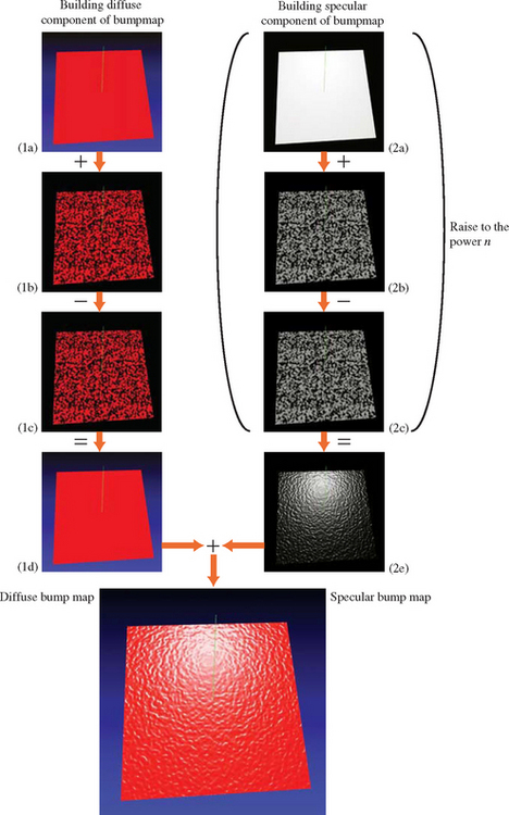
1. Render the bump map texture.
2. Shift the texture coordinates at the vertices by s′, t′.
3. Rerender the bump map texture, subtracting from the first image.
Consider a 1D bump map for simplicity. The map only varies as a function of s. Assuming that the height values of the bump map can be represented as a height function F(s), then the three-step process computes the following: F(s) − F(s + Δs)/Δs. If the delta is one texel in s, then the resulting texture coordinate is ![]() , where w is the width of the texture in texels (see Figure 15.14). This operation implements a forward difference of F, approximating the first derivative of F if F is continuous.
, where w is the width of the texture in texels (see Figure 15.14). This operation implements a forward difference of F, approximating the first derivative of F if F is continuous.
In the 2D case, the height function is F(s, t), and performing the forward difference in the directions of s′ and t′ evaluates the derivative of F(s, t) in the directions s′ and t′. This technique is also used to create embossed images.
This operation provides the values used for the first two addends shown in Equation 15.2. In order to provide the third addend of the dot product, the process needs to compute and add the transformed z component of the light vector. The tangent space transform in Equation 15.3 implies that the transformed z component of L′ is simply the inner product of the vertex normal and the light vector, ![]() . Therefore, the z component can be computed using OpenGL to evaluate the diffuse lighting term at each vertex. This computation is performed as a second pass, adding to the previous results. The steps for diffuse bump mapping are summarized:
. Therefore, the z component can be computed using OpenGL to evaluate the diffuse lighting term at each vertex. This computation is performed as a second pass, adding to the previous results. The steps for diffuse bump mapping are summarized:
1. Render the polygon with the bump map texture, modulating the polygon color. The polygon color is set to the diffuse reflectance of the surface. Lighting is disabled.
2. Find N, T, and B at each vertex.
3. Use the vectors to create a transformation.
4. Use the matrix to rotate the light vector L into tangent space.
5. Use the rotated x and y components of L to shift the s and t texture coordinates at each polygon vertex.
6. Rerender the bump map textured polygon using the shifted texture coordinates.
7. Subtract the second image from the first.
8. Render the polygon with smooth shading, with lighting enabled, and texturing disabled.
Using the accumulation buffer can provide reasonable accuracy. The bump-mapped objects in the scene are rendered with the bump map, rerendered with the shifted bump map, and accumulated with a negative weight (to perform the subtraction). They are then rerendered using Gouraud shading and no bump map texture, and accumulated normally.
The process can also be extended to find bump-mapped specular highlights. The process is repeated using the halfway vector (H) instead of the light vector. The halfway vector is computed by averaging the light and viewer vectors ![]() . The combination of the forward difference of the bump map in the direction of the tangent space H and the z component of H approximate N · H. The steps for computing N · H are as follows.
. The combination of the forward difference of the bump map in the direction of the tangent space H and the z component of H approximate N · H. The steps for computing N · H are as follows.
1. Render the polygon with the bump map textured on it.
2. Find N, T, and B at each vertex.
3. Use the vectors to create a rotation matrix.
4. Use the matrix to rotate the halfway vector H into tangent space.
5. Use the rotated x and y components of H to shift the s and t texture coordinates at each polygon vertex.
6. Rerender the bump-map-textured polygon using the shifted texture coordinates.
7. Subtract the second image from the first.
8. Render the polygon Gouraud shaded with no bump map texture. This time use H instead of L as the light direction. Set the polygon color to the specular light color.
The resulting N·H must be raised to the shininess exponent. One technique for performing this exponential is to use a color table or pixel map to implement a table lookup of f(x) = xn. The color buffer is copied onto itself with the color table enabled to perform the lookup. If the object is to be merged with other objects in the scene, a stencil mask can be created to ensure that only pixels corresponding to the bump-mapped object update the color buffer (Section 9.2). If the specular contribution is computed first, the diffuse component can be computed in place in a subsequent series of passes. The reverse is not true, since the specular power function must be evaluated on N · H by itself.
Blending
If the OpenGL implementation doesn’t accelerate accumulation buffer operations, its performance may be very poor. In this case, acceptable results may be obtainable using framebuffer blending. The subtraction step can produce intermediate results with negative values. To avoid clamping to the normal [0, 1] range, the bump map values are scaled and biased to support an effective [-1, 1] range (Section 3.4.1). After completion, of the third pass, the values are converted back to their original 0 to 1 range. This scaling and biasing, combined with fewer bits of color precision, make this method inferior to using the accumulation buffer.
Bumps on Surfaces Facing Away from the Light
Because this algorithm doesn’t take self-occlusion into account, the forward differencing calculation will produce “lights” on the surface even when no light is falling on the surface. Use the result of L · N to scale the shift so that the bump effect tapers off slowly as the surface becomes more oblique to the light direction. Empirically, adding a small bias (.3 in the authors’ experiments) to the dot product (and clamping the result) is more visibly pleasing because the bumps appear to taper off after the surface has started facing away from the light, as would actually happen for a displaced surface.
15.10.4 Limitations
Although this technique does closely approximate bump mapping, there are limitations that impact its accuracy.
Bump Map Sampling
The bump map height function is not continuous, but is sampled into the texture. The resolution of the texture affects how faithfully the bump map is represented. Increasing the size of the bump map texture can improve the sampling of high-frequency height components.
Texture Resolution
The shifting and subtraction steps produce the directional derivative. Since this is a forward differencing technique, the highest frequency component of the bump map increases as the shift is made smaller. As the shift is made smaller, more demands are made of the texture coordinate precision. The shift can become smaller than the texture filtering implementation can handle, leading to noise and aliasing effects. A good starting point is to size the shift components so that their vector magnitude is a single texel.
Surface Curvature
The tangent coordinate axes are different at each point on a curved surface. This technique approximates this by finding the tangent space transforms at each vertex. Texture mapping interpolates the different shift values from each vertex across the polygon. For polygons with very different vertex normals, this approximation can break down. A solution would be to subdivide the polygons until their vertex normals are parallel to within an error limit.
Maximum Bump Map Slope
The bump map normals used in this technique are good approximations if the bump map slope is small. If there are steep tangents in the bump map, the assumption that the perturbed normal is length one becomes inaccurate, and the highlights appear too bright. This can be corrected by normalizing in fourth pass, using a modulating texture derived from the original bump map. Each value of the texel is one over the length of the perturbed normal: ![]() .
.
15.11 Normal Maps
Normal maps are texture maps that store a per-pixel normal vector in each texel. The components of the normal vector are stored in the R, G, and B color components. The normal vectors are in the tangent space of the object (see Section 15.10.2). Relief shading, similar to bump mapping, can be performed by computing the dot product N · L using the texture combine environment function. Since the computation happens in the texture environment stage, the colors components are fixed point numbers in the range [0, 1]. To support computations of inputs negative components, the dot product combine operation assumes that the color components store values that are scaled and biased to represent the range [-1, 1]. The dot product computation is
producing a result that is not scaled and biased. If the dot product is negative, the regular [0, 1] clamping sets the result to 0, so the dot product is N · L rather than N · L.
To use normal maps to perform relief shading, first a tangent-space biased normal map is created. To compute the product N · L, the tangent space light vector L is sent to the pipeline as a vertex color, using a biased representation. Since interpolating the color components between vertices will not produce correctly interpolated vectors, flat shading is used. This forces the tangent-space light vector to be constant across the face of each primitive. The texture environment uses GL_COMBINE for the texture environment function and GL_DOT3_RGB for the RGB combine operation. If multiple texture units are available, the resulting diffuse intensity can be used to modulate the surface’s diffuse reflectance stored in a successive texture unit. If there isn’t a texture unit available, a two-pass method can be used. The first pass renders the object with diffuse reflectance applied. The second pass renders the object with the normal map using framebuffer blending to modulate the stored diffuse reflectance with the computed diffuse light intensity.
If programmable pipeline support is available, using normal maps becomes simple. Direct diffuse and specular lighting model computations are readily implemented inside a fragment program. It also provides an opportunity to enhance the technique by adding parallax to the scene using offset mapping (also called parallax mapping) (Welsh, 2004). This adds a small shift to the texture coordinates used to look up the diffuse surface color, normal map, or other textures. The offset is in the direction of the viewer and is scaled and biased by the height of the bump, using a scale and bias of approximately 0.04 and 0.02.
15.11.1 Vector Normalization
For a curved surface, the use of a constant light vector across the face of each primitive introduces visible artifacts at polygon boundaries. To allow per-vertex tangent-space light vector to be correctly interpolated, a cube map can be used with a second texture unit. The light vector is issued as a set of (s, t, r) texture coordinates and the cube map stores the normalized light vectors. Vectors of the same direction index the same location in the texture map. The faces of the cube map are precomputed by sequencing the two texture coordinates for the face through the integer coordinates [0, M − 1] (where M is the texture size) and computing the normalized direction. For example, for the positive X face at each y, z pair,
and the components of the normalized vector N are scaled and biased to the [0, 1] texel range. For most applications 16 × 16 or 32×32 cube map faces provide sufficient accuracy.
An alternative to a table lookup cube map for normalizing a vector is to directly compute the normalized value using a truncated Taylor series approximation. For example, the Taylor series expansion for N′ = N/![]() N
N![]() is
is
which can be efficiently implemented using the combine environment function with two texture units if the GL_DOT3_RGB function is supported. This approximation works best when interpolating between unit length vectors and the deviation between the two vectors is less than 45 degrees. If the programmable pipeline is supported by the OpenGL implementation, normalization operations can be computed directly with program instructions.
15.12 Bump-mapped Reflections
Bump mapping can be combined with environment mapping to provide visually interesting perturbed reflections. If the bump map is stored as displacements to the normal ![]() rather than a height field, the displacements can be used as offsets added to the texture coordinates used in a second texture. This second texture represents the lighting environment, and can be the environment-mapped approximation to Phong lighting discussed in Section 15.4 or an environment map approximating reflections from the surface (as discussed in Section 17.3.4).
rather than a height field, the displacements can be used as offsets added to the texture coordinates used in a second texture. This second texture represents the lighting environment, and can be the environment-mapped approximation to Phong lighting discussed in Section 15.4 or an environment map approximating reflections from the surface (as discussed in Section 17.3.4).
The displacements in the “bump map” are related to the displacements to the normal used in bump mapping. The straightforward extension is to compute the reflection vector from displaced normals and use this reflection vector to index the environment map. To simplify hardware design, however, the displaced environment map coordinates are approximated by applying the bump map displacements after the environment map coordinates are computed for the vertex normals. With sphere mapping, the error introduced by this approximation is small at the center of the sphere map, but increases as the mapped normal approaches the edge of the sphere map. Images created with this technique look surprisingly realistic despite the crudeness of the approximation. This feature is available through at least one vendor-specific extension ATI_envmap_bumpmap.
15.13 High Dynamic Range Lighting
In Section 12.9 we introduced the idea of high dynamic range images (HDR images). These images are capable of storing data over a much larger range than a typical 8-bit-per-component color buffer. The section also describes the process of tone mapping, which maps the components of an HDR image to the component resolutions of a typical display device. A natural outgrowth of being able to capture and store an HDR image is to generate scenes with HDR lighting. This facilitates the implementation of physically based rendering using spectral radiance for real llumination sources. Alternatively, HDR scenes can also be rendered using image-based lighting derived from HDR images (Debevec, 2002).
The simplest way to implement HDR image-based lighting is to capture the environment as an HDR environment map, called a radiance map. Sphere map environment maps of HDR data are termed light probes and can be captured with a fish-eye lens or by photographing a chrome ball from a distance, just like a sphere environment map. Special processing is required to recover the HDR values; it is described in detail by Paul Debevec in (Debevec, 1997) and (Debevec, 2002). Lighting a scene with the HDR environment is similar to other environment mapping techniques; the system must be capable of processing HDR color values, however, so fragment programs and HDR texture image formats and color buffers are required. The end result is an HDR image that must be tone mapped to map the HDR pixel values to a displayable range, as described in Section 12.9.2.
15.13.1 Bloom and Glare Effects
The human visual system response to high-luminance sources results in several visible effects, including glare, lenticular halos, and bloom (Spencer, 1995). Some of these effects can be simulated as part of an HDR rendered scene. They are performed as a postprocess on the HDR rendered scene, called a “bright pass.”
The first step uses the tone-mapping operator to segment the scene into bright and dim parts. To extract the bright part of the scene, the curve-based tone mapping operator from Section 12.9.2 is modified and applied in pieces. First, the log-average luminance is computed and colors are scaled by the a/Lavg, and then the dim pixels are subtracted away using a threshold value of 5, clamping the result to zero. Finally, the remaining “bright” values are scaled by 1/(10 + Lscale(x, y)) to isolate the light sources. The values of 5 and 10 are empirically chosen, with 5 representing the threshold luminance for dark areas and the offset value 10 defining the degree of separation between light and dark areas. Once the bright image is computed, it is blurred using a Gaussian or other filter and the result is added to the tone-mapped scene.
The bright image can be used for other glare or halo effects by locating the positions of the light source and sampling specific patterns (circles, crosses, and so on) and smearing them along the pattern. The result is added back to the orginal scene.
15.14 Global Illumination
The lighting models described thus far have been growing progressively more sophisticated. However, capturing the effects of complex interreflections, area light sources, and so on is increasingly difficult using individual light sources. Environment maps capture some of the information in a more complex environment, but the subtleties of real lighting are often better captured using a global illumination model. Global illumination models using radiosity or ray tracing are generally too computationally complex to perform in real time. However, if the objects and light sources comprising the environment are static, it is possible to perform the global illumination calculations as a preprocessing step and then display the results interactively. Such an approach is both practical and useful for applications such as architectural walkthroughs. The technique is typically employed for diffuse illumination solutions since view-independent (ideal) diffuse illumination can be represented as a single value (color) at each object vertex.
Many of the techniques for the display of precomputed global illumination parameterize the radiance transfer with a set of basis functions such as wavelets or spherical harmonics. This allows the lighting contribution to be factored out, so that at display time a dynamic lighting environment projected onto the same basis can be used to light the scene efficiently. This computation is usually with an N dimensional dot product, where N ≤ the number of basis functions used to parameterize the solution. Details for these techniques are beyond the scope of this book, but we will outline some methods that do not require an extended mathematical discussion.
15.14.1 Virtual Light Technique
Walter et al. (Walter, 1997) describe a method for rendering global illumination solutions that contain view-independent directionally variant lighting effects. The specular term in the OpenGL lighting model is used to approximate the directionally varying lighting information, and the emissive term is used to approximate the directionally invariant illumination (diffuse illumination). In this method, a set of OpenGL lights is treated as a set of basis functions that are summed together, whereas the object is rendered to yield a more general directional distribution. The OpenGL light parameters, such as position or intensity coefficients, have no relationship to the light sources in the original model, but instead serve as a compact representation for the directional illumination of an object. Each rendered object has its own set of lights, called virtual lights.
The method works on a global illumination solution, which stores a number of samples of the directionally varying illumination at each object vertex. The parameters for the virtual lights of a particular object are determined using a fitting procedure consisting of a number of heuristics. The main idea is to produce a set of solutions for a number of specular exponent values and then choose the exponent value that minimizes the mean-squared error using a least squares method. A solution at a given exponent value is determined as follows.
1. Choose a specular exponent value.
2. Find the vertex on the object with the largest directional radiance.
3. Choose a light direction to align the specular lobe with this brightest direction.
4. Choose an intensity coefficient to match the radiance at the point on the object.
5. Compute the specular contribution at other points on the object and subtract from the radiance.
6. Repeat steps 2 through 5 using updated object radiance until all lights have been used.
7. At each vertex, compute the specular and emission coefficients using a least squares fit.
Once the lighting parameters have been determined, the model is rendered using the glLight and glMaterial commands to set the directional light parameters and specular exponent for each object. The glMaterial command is used to set the specular reflectance and emitted intensity at each vertex. The rendering speed for the model is limited by its geometric complexity and of the OpenGL implementation’s ability to deal with multiple light sources and material changes at each vertex. Rendering performance may be improved by rendering in multiple passes to limit the number of active lights or the number of material parameter changes in each pass. For example, use glColorMaterial and glColor to change only the emitted intensity or specular reflectance in each pass and framebuffer blending can then be used to sum the results together.
15.14.2 Combining OpenGL Lighting with Radiosity
Radiosity solutions produce accurate global illumination solutions for diffuse reflections (Cohen, 1993). While the solutions are view independent, they are computationally expensive, so their usefulness tends to be limited to static scenes. They have another limitation, they can’t model specular reflections, so separate processing must be done to add them. The hardware lighting equations supported by OpenGL are fast, and provide adequate realism for direct lighting of objects. A hybrid solution can combine the best of both radiosity and OpenGL lighting. This technique creates realistic scenes with both diffuse and specular reflections that are viewer dependent and insensitive to small changes in object position.
Computing radiosity is a recursive process. Each step consists of processing each surface, computing the incoming radiosity from each visible surface in the scene, then updating the emitted radiosity of the surface. This process is repeated until the radiosity values of the surfaces converge. The first step of this process consists of setting the radiosity of the illumination sources of the room. Thus, the first radiosity iteration computes the contributions of surfaces directly illuminated from the scene’s light sources.
The hybrid approach computes the radiosity equation, then subtracts out the radiosity contributes from this first step. What’s left is the indirect illumination caused by object interreflection. The objects in the scene are colored using this radiosity result, then lighted using standard OpenGL lighting techniques. The OpenGL lighting provides the missing direct illumination to the scene. The lighting equation is parameterized to provide no ambient illumination, since the radiosity computations supply a more accurate solution.
This technique has several advantages. Since normal OpenGL lighting provides the direct specular and diffuse lighting, the viewer-dependent parts of the scene can be rendered quickly, once the initial radiosity computations have been completed. The radiosity results themselves are more robust, since they only contribute lighting effects from object interreflections. Viewed as light sources, objects in the scene tend to have large areas, so the amount of incident light falling on any given object is fairly insensitive to its position in the scene. These effects are also a smaller percentage of the total lighting contribution, so they will still “look right” longer as the object moves, since the direct part of the lighting contribution is taking object position into account.
As a scene is dynamically updated, at some point the radiosity errors will become noticeable, requiring that the radiosity equations be recomputed. Since these errors accumulate slowly, this cost can be amortized over a large number of frames. Small objects can move significantly without large error, especially if they are not very near large objects in the scene. Other techniques mentioned in this book can be combined with this one to improve the realism of OpenGLs direct illumination, since the radiosity contribution and the direct illumination contribution are orthogonal. See (Diefenbach, 1997) for more details on this technique.
15.14.3 Ambient Occlusion
Ambient occlusion is a scalar value recorded at every surface point indicating the average amount of self-occlusion occurring at the point on the surface. It measures the extent to which a location on the surface is obscured from surrounding light sources. It is used to approximate self-shadowing and adds realism to lighting by mimicking the effects of indirect light sources such as sky, ground, walls, and so on.
To use ambient occlusion in interactive rendering, the occlusion term is computed as a preprocessing step and relies on the geometry being rigid and the lighting constant to avoid recomputing the occlusion information. Like other light transport modeling methods, this one is restricted to diffuse surfaces; i.e. view-independent lighting. Ambient occlusion is computed for each object independently, not for the entire scene, so objects can undergo separate rigid transformations such as rotation and translation while using the same ambient occlusion map.
Conceptually, the ambient occlusion at a surface point is computed by casting rays sampling the hemisphere over the surface point (see Figure 15.15). The rays themselves are used to compute visibility. The point is partially occluded if the ray interesects another part of the object geometry as it extends outward toward a hemisphere bounding the object.
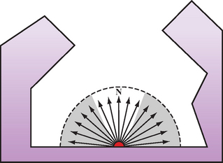
If the rays are uniformly distributed across the hemisphere; the single ambient occlusion value is a weighted average of the visibility results (Vp(ω)) using hemispherical integration.
One method for weighting the samples uses the cosine of the angle between the surface normal at the point and the direction of the sample ray. This can be computed more efficiently by using a cosine distribution of sample rays, summing the results directly (Monte Carlo integration).
The results of computing the occlusion value at different sample points are combined to form an ambient occlusion map. Like other lighting techniques, ambient occlusion maps may be sampled at different frequencies (for example, at each vertex, or at regular points on the object surface). The goal is to have the sample rate match the rate of change of the occlusion detail on the object.
The ambient occlusion map is applied during rendering by modulating the result of diffuse lighting computations with the ambient occlusion term. For occlusion values sampled at vertices, the occlusion term can be included in the material reflectance for the vertex (using color material or a vertex program). High-density occlusion maps are used as textures and also modulate the result of the diffuse lighting computation. An additional improvement to the scheme replaces the surface normal with a “bent norma l”-the average unoccluded direction. Figure 15.16 illustrates a per-pixel occlusion Map applied to a sample object.
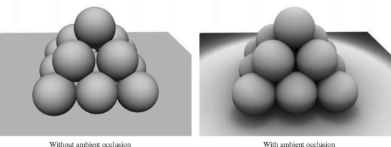
Incorporating ambient occlusion enhances flat illumination by adding extra definition. It is efficient and relatively low cost techique to add to the rendering step. The only downside is the requirement for precomputation of the map. With some cleverness, however, the precomputation can also be hardware accelerated using the OpenGL pipeline (Whitehurst, 2003; Hill, 2004; Fernando, 2004).
15.15 Summary
Lighting continues to be one of the most actively researched areas in computer graphics. New lighting models and methods for emulating surface characteristics and light transport continue to be developed. Texture mapping combined with the programmable fragment pipeline greatly increases the range of lighting models that can be im plem ented within the OpenGL pipeline. This chapter covers only a subset of frequently used lighting algorithms. They represent different trade-offs in terms of visual quality and com putational cost; their applicability is dependent on both the needs of the application and the capabilities of the OpenGL im plementation.
1Recall that A · B = max(0, A · B) is the clamped inner product as described in Section 3.3
2Multitexture and the combine texture environment are part of OpenGL 1.3 or available as extensions. Vertex and fragment programs are available as the extensions ARB_vertex_program and ARB_fragment_program.
3Added in OpenGL 1.2.
4A core feature in OpenGL 1.4 and available as the ARB_texture_mirrored_repeat extension.