
CHAPTER 5
Formatting a Pivot Table
In this chapter, you'll continue to work with the WorkOrders pivot table. First, download and open the sample file WorkOrders_02.xlsx. You'll add formatting to the pivot table to enhance the data presentation. With suitable formatting, you can make the pivot table easier to read, and you can highlight specific data. You'll also apply, modify, and create pivot table styles and themes in order to make formatting consistent throughout your workbook.
Controlling the Report Layout
First you'll experiment with the overall layout options for the pivot table. Three layouts are available for pivot tables: Compact Form, Outline Form, and Tabular Form. When you create a new pivot table, it is automatically formatted with the Compact Form layout. You'll apply the other two layouts to your pivot table and then reapply the Compact Form layout so you can see the differences.
Applying Outline Form Layout
The first layout you'll apply is the Outline Form layout to see how it differs from the Compact Form layout. Before changing the report layout, you'll turn on the subtotals so you can also see how they are affected by the layout changes:
- Select a cell in the pivot table.
- On the Ribbon, under the PivotTable Tools tab, click the Design tab.
- At the far left, in the Layout group, click the Subtotals command, and click Show All Subtotals at Top of Group.
- In the Layout group, click the Report Layout command, and click Show in Outline Form (see Figure 5-1).
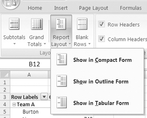
Figure 5-1. Report Layout menu options
After you've applied the Outline Form layout, the row labels change from using one column for all the labels to using a separate column for each field (see Figure 5-2). In the Compact Form layout, the labels are all shown in column A, under the heading Row Labels.In Outline Form layout, there are two headings—LeadTech2 is in cell A3, and LeadTech is in cell B3. Below each heading are the labels for the field that is named in the heading cell.
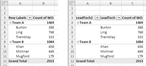
Figure 5-2. Compact Form (on the left) and Outline Form (on the right) layouts
The Outline Form layout may be useful when you want to show all the field names as heading labels and aren't concerned about the width of the pivot table.
Applying Tabular Form Layout
Next, you'll apply the Tabular Form layout to the pivot table to see how it differs from the Outline Form layout:
- Select a cell in the pivot table.
- On the Ribbon, under the PivotTable Tools tab, click the Design tab.
- At the far left, in the Layout group, click the Report Layout command.
- Click Show in Tabular Form.
After the Tabular Form layout is applied, the first item for each field starts in the first available row (see Figure 5-3). As in Outline Form layout, there are two headings—LeadTech2 is in cell A3, and LeadTech is in cell B3. Below each heading are the labels for the field that is named in the heading cell.
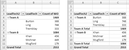
Figure 5-3. Outline Form (on the left) and Tabular Form (on the right) layouts
Note In the Tabular Form layout, the subtotals are at the bottom of the group, even though you selected the option to show the subtotals above the group.
If you remove the subtotals, the Tabular Form layout will require fewer rows than the Outline Form layout, because it doesn't add an extra row for each group heading, such as Team A and Team B. The Tabular Form layout may be useful when you want to show all the field names as heading labels and aren't concerned about the width of the pivot table but want to reduce the number of rows.
Applying Compact Form Layout
Next, you'll apply the Compact Form layout to the pivot table to return the pivot table to its original layout:
- Select a cell in the pivot table.
- On the Ribbon, under the PivotTable Tools tab, click the Design tab.
- At the far left, in the Layout group, click the Report Layout command.
- Click Show in Compact Form.
After the Compact Form layout is applied, the headings for LeadTech2 and LeadTech disappear. The row labels are all shown in column A, under the heading Row Labels, as they were originally (see the Compact Form layout in Figure 5-2). The indentation differentiates the sets of items. Also, because you've removed the Tabular Form layout, the subtotals are now visible at the top of each group.
Adding Blank Rows in the Layout
To add some whitespace to a pivot table and make it easier to distinguish where items end, you can change a setting to add blank rows to the layout. You'll add blank rows to your pivot table to see the effect:
- Select a cell in the pivot table.
- On the Ribbon, under the PivotTable Tools tab, click the Design tab.
- At the far left, in the Layout group, click the Blank Rows command.
- Click Insert Blank Line After Each Item (see Figure 5-4).
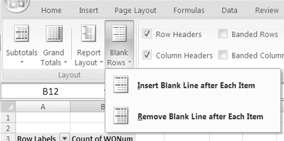
Figure 5-4. Blank Rows options
The pivot table now has a blank row after each item in the outer fields in the Row Labels area. Adding this whitespace may make the pivot table easier to read, especially if it is large or is crowded with large numbers.
If you've added blank rows to the pivot table, later you can remove the rows by using the Blank Rows command on the Ribbon. You'll remove the blank rows that you added:
- Select a cell in the pivot table.
- On the Ribbon, under the PivotTable Tools tab, click the Design tab.
- At the far left, in the Layout group, click the Blank Rows command.
- Click Remove Blank Line After Each Item.
This removes the blank row after each item and reduces the number of rows in the pivot table.
Using a Pivot Table Style
To quickly and easily format a pivot table, you can apply a pivot table style. If you change the pivot table layout, the pivot table style formatting will adjust to the revised layout, so formatting such as alternating shaded rows will display correctly when rows are added or removed from the pivot table layout.
In Chapter 3 you applied a pivot table style. In this chapter, you'll modify and create pivot table styles and see how the styles work in conjunction with other formatting features in Excel. To get started, you'll apply one of the existing styles:
- Select a cell in the pivot table.
- On the Ribbon, under the PivotTable Tools tab, click the Design tab.
- Click the More arrow at the bottom right of the PivotTable Styles group.
- In the Medium section of the PivotTable Style gallery, click Pivot Style Medium 8.
Tip As you point to the styles in the Pivot Table Style gallery, the style will be previewed in the active pivot table.
The style you applied has medium gray fill in the column headings, light gray fill in the row headings, and borders on the grand total row. Next, you'll use other commands on the Ribbon to modify the selected style.
Adding Row and Column Shading
In a large pivot table it may be difficult to visually connect a label at the far left or top of the pivot table to a number in the center of the Values area. To help users follow a wide row or long column of data, you can use the Banded Rows and Banded Columns commands on the PivotTable Design tab.
Applying Banded Rows to the Pivot Table
In your pivot table, you'll add Banded Rows to make it easier to follow the data across the row for each technician:
- Select a cell in the pivot table.
- On the Ribbon, under the PivotTable Tools tab, click the Design tab.
- In the PivotTable Style Options group, click the Banded Rows command to add a check mark to the option (see Figure 5-5).
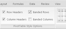
Figure 5-5. Banded Rows command
In the pivot table, the formatting changes to include light gray borders between the rows. In the PivotTable Styles group, the style samples have changed to include banded rows.
Tip For some pivot table styles, such as PivotStyle Medium 15, applying the Banded Rows command will create alternating shaded rows, instead of row borders.
- To see the benefit of the row banding, in the PivotTable Field List pane, drag the District field to the Column Labels area.
In the wider pivot table, the gray borders help you read across the rows, connecting the technician names to the data in all the columns.
Applying Banded Columns to the Pivot Table
If a pivot table has long columns, the Banded Columns feature may make it easier to read. Before applying this feature, you'll add another field to the Row Labels area to add more rows:
- To increase the number of rows in the pivot table, in the PivotTable Field List pane, add a check mark to the Service field. It is added to the Row Labels area, below the LeadTech field.
- On the Ribbon, under the PivotTable Tools tab, click the Design tab.
- In the PivotTable Style Options group, click the Banded Columns command to add a check mark to the option.
In pivot table, the formatting changes to include gray borders between the columns. In the PivotTable Styles group, the style samples have changed to include banded columns.
Tip For some pivot table styles, such as PivotStyle Medium 15, applying the Banded Columns command will create alternating shaded columns, instead of column borders.
Formatting the Row and Column Headers
Another option you can turn on or off in a pivot table style is special formatting for the row headers and column headers. When you create a pivot table, formatting for row headers and column headers is turned on by default.
Removing Row Header Formatting
You'll turn off the row header formatting in your pivot table to see the effect, and then you'll turn it back on:
- Select a cell in the pivot table.
- On the Ribbon, under the PivotTable Tools tab, click the Design tab.
- In the Options group, click the Row Headers command to remove the check mark from the option (see Figure 5-6).
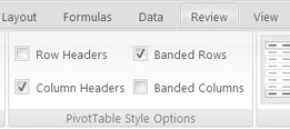
Figure 5-6. Row Headers command
In your pivot table, the formatting for the row label headers is removed, and the cells are formatted like the other cells in the body of the pivot table. On the Ribbon, in the PivotTable Styles group, some of the style samples have changed to remove the row header formatting.
- To turn the row header formatting on again, click the Row Headers command to add a check mark.
Removing Column Header Formatting
You'll turn off the column header formatting in your pivot table to see the effect, and then you'll turn it back on:
- On the Ribbon, under the PivotTable Tools tab, click the Design tab.
- In the Options group, click the Column Headers command to remove the check mark from the option.
In the pivot table, the formatting is removed from the column labels, and in the PivotTable Styles group, some of the style samples have changed to remove the column header formatting.
- To turn the column header formatting on again, click the Column Headers command to add a check mark.
Removing a Pivot Table Style
After applying a pivot table style to a pivot table, you may want to clear the style and start over, or you simply might want to work with an unformatted pivot table. You'll remove the pivot table style from your pivot table to prepare for creating your own pivot table style:
- Select a cell in the pivot table.
- On the Ribbon, under the PivotTable Tools tab, click the Design tab.
- Click the More arrow at the bottom right of the PivotTable Styles group.
- At the bottom left of the gallery, click Clear to remove the pivot table style (see Figure 5-7).
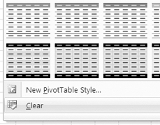
Figure 5-7. Clearing the pivot table style
This removes the pivot table style from the pivot table, and the cells have no fill color, bold font, or colored borders; they have only the formatting that was manually applied to the cells. Checking the options in the PivotTable Style Options group on the Ribbon has no effect on the pivot table, because no style is applied.
Tip A pivot table style, None, appears at the top left in the PivotTable Styles group on the Ribbon. You can use it to clear the pivot table style, just as you would use the Clear command.
Creating a Pivot Table Style
In addition to using the built-in pivot table styles, you can create and apply your own pivot table styles, either from scratch or based on an existing pivot table style. You'll create a pivot table style from scratch and apply it to your pivot table:
- Select a cell in the pivot table.
- On the Ribbon, under the PivotTable Tools tab, click the Design tab.
- Click the More arrow at the bottom right of the PivotTable Styles group.
- Click New PivotTable Style (shown earlier in Figure 5-7).
- In the New PivotTable Quick Style dialog box, type WorkOrders in the Name box as the name for your new style (see Figure 5-8).
Tip In the Preview section of the New PivotTable Quick Style dialog box, you can see a sample of the formatting as you create it.
Figure 5-8. The New PivotTable Quick Style dialog box
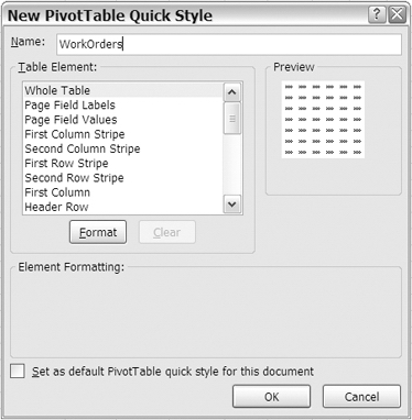
- In the Table Element list, scroll down to Grand Total Row, click to select it, and then click the Format button.
Note The Grand Total Row element is the row at the bottom of the pivot table. It is different from the Grand Totals for Rows element in the column at the far right of the pivot table.
- In the Format Cells dialog box, click the Fill tab, and select a background color for the grand total row.
- Click the Border tab, select a line style and line color, and then select borders for the grand total row.
- Click the Font tab, and select Bold as the font style.
- Click the OK button to return to the New PivotTable Quick Style dialog box, where the formatted grand total row is listed with a bold font.
Tip Click a formatted table element, and you can view a description of its formatting in the Element Formatting section of the New PivotTable Quick Style dialog box.
- Repeat steps 6 to 10 to format the Header Row and Row Subheading 1 table elements.
- Click the OK button to close the New PivotTable Quick Style dialog box.
Note The new pivot table style is not automatically applied to the active pivot table.
The pivot table style you created may be visible on the Ribbon, under the PivotTable Tools tab, in the PivotTable Styles group on the Design tab. It is also added to a Custom section of the PivotTable Styles gallery (see Figure 5-9).
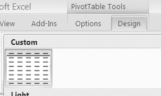
Figure 5-9. The Custom pivot table styles on the Ribbon
Applying a Custom Pivot Table Style
After you have created a custom pivot table style, you can apply it to your pivot table. You'll apply the WorkOrders pivot table style to your pivot table:
- Select a cell in the pivot table.
- On the Ribbon, under the PivotTable Tools tab, click the Design tab.
- Click the WorkOrders style in the PivotTable Styles group (see Figure 5-10).
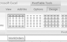
Figure 5-10. The new pivot table style on the Ribbon
The WorkOrders custom pivot table style is applied to your pivot table, with the formatting you selected when creating the style.
Modifying a Custom PivotTable Style
After you have created a custom pivot table style, you can modify it. You'll modify the WorkOrders custom pivot table style to remove formatting from one table element and to add formatting to another table element:
- Select a cell in the pivot table.
- On the Ribbon, under the PivotTable Tools tab, click the Design tab.
- Right-click the WorkOrders custom style in the PivotTable Styles group, and click Modify (see Figure 5-11).
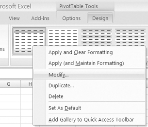
Figure 5-11. Modifying the custom pivot table style
- In the Modify PivotTable Quick Style dialog box, select Row Subheading 1 in the Table Element list, and click Clear to clear its formatting.
- Select First Row Stripe in the Table Element list, and in the Stripe Size drop-down list, choose 2.
- Click the Format button, and on the Fill tab, select a background color.
- Click OK to close the Format Cells dialog box, and you'll see the stripe in the preview section of the Modify PivotTable Quick Style dialog box. Because you set the stripe size to 2, there are two shaded rows and then a row with no fill color.
- Click OK to close the Modify PivotTable Quick Style dialog box.
Because the WorkOrders style is applied to the active pivot table, you'll automatically see the custom style's changes displayed in the pivot table.
Duplicating a Pivot Table Style
You can duplicate a built-in or custom pivot table style and modify the duplicate copy to create a new pivot table style. Earlier, you created the WorkOrders custom pivot table style from scratch. Now you'll duplicate one of the built-in pivot table styles and then modify it to create a new style:
- Select a cell in the pivot table.
- On the Ribbon, under the PivotTable Tools tab, click the Design tab.
- In the PivotTable Styles gallery, in the Dark section, right-click Pivot Style Dark 11, and click Duplicate (see Figure 5-12).
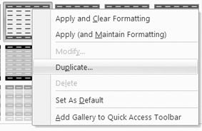
Figure 5-12. Duplicating a pivot table style
- Type Dark Green Header as a name for the new pivot table style.
- In the Table Element list, select Header Row, and format it with dark green background color instead of black.
- When finished, click the OK button, and then apply the Dark Green Header style to your pivot table.
The new style is applied to the pivot table, with the formatting changes you made.
Deleting a Custom Pivot Table Style
If you no longer need a custom pivot table style, you can delete it. You'll delete the Dark Green Header style you just created:
- Select a cell in the pivot table.
- On the Ribbon, under the PivotTable Tools tab, click the Design tab.
- In the PivotTable Styles gallery, right-click the Dark Green Header custom style, and click Delete.
- In the alert message, click the OK button to confirm the deletion (see Figure 5-13).
Figure 5-13. Deleting the custom pivot table style
Because your pivot table had the Dark Green Header custom style applied, when you deleted that style, the style was automatically removed from your pivot table. You can apply a different style from the PivotTable Style gallery.
- On the Ribbon, in the PivotTable Styles gallery, click the WorkOrders custom style to apply it to your pivot table.
Using Themes
Another feature in Excel 2007 that affects the formatting is document themes. Each theme is a collection of colors, fonts, and visual effects you can share between Excel and other Microsoft Office applications. You can use the existing themes, create new themes, or modify the built-in themes. In the following sections, you'll experiment with document themes to help you understand their impact on pivot table formatting.
Viewing the Current Theme
First, you'll check the theme information for your workbook to see what theme is currently applied and what its settings are. Later, you'll apply a different theme to see what changes occur.
- On the Ribbon, click the Page Layout tab.
- In the Themes group, point to the Themes command, and the tool tip will show Office Theme as the name of the current theme (see Figure 5-14).
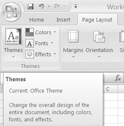
Figure 5-14. Current theme
Viewing the Theme Colors
Next, you'll see the colors that are associated with each theme and view the color palette for the current theme:
- In the Themes group, click Colors to open the color list, where the Office colors are shown as selected (see Figure 5-15). To close the list, click the Colors command again.
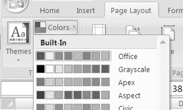
Figure 5-15. Current colors
- To see more of the Office Theme color palette, on the Ribbon, click the Home tab, and then click the arrow on the Fill Color command. The Fill Color palette shows the theme colors in the first row of colors (see Figure 5-16). The colors in the rows below are lighter and darker versions of the theme colors.
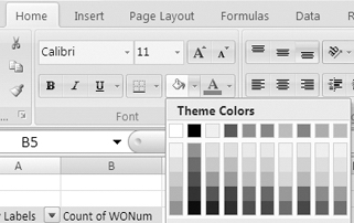
Figure 5-16. Theme colors in the Fill Color palette
The first four theme colors are used for text and backgrounds. The next six colors are the accent colors and are also used for the pivot table styles.
Viewing the Theme Fonts
Next, you'll view the fonts associated with the current theme. A theme has two fonts, one for headings and one for the body text.
- On the Ribbon, click the Page Layout tab.
- In the Themes group, click the Fonts command to open the list of fonts (see Figure 5-17).
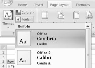
Figure 5-17. Current theme fonts
The Office fonts are selected and show that Cambria is the Headings font and Calibri is the Body font. These fonts are also visible in the Font drop-down list on the Home tab on the Ribbon (see Figure 5-18). In your pivot table, Calibri, the Body font from the Office theme, is used.
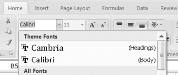
Figure 5-18. Theme fonts in the Font drop-down list on the Home tab
Viewing the Theme Effects
Finally, you'll view the effects associated with the current theme. The effects are used in charts and shapes, so if you create a pivot chart, its appearance will be affected by the current theme's effects.
- On the Ribbon, click the Page Layout tab.
- In the Themes group, click the Effects command to open the list of effects (see Figure 5-19).
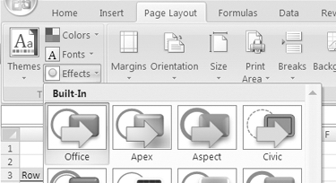
Figure 5-19. Current theme effects
The Office theme effects are selected and show the line thickness, fill type, and beveling that would be used for charts and shapes.
Applying a Theme
To change the look of your pivot table, you'll apply a different theme to see what changes occur:
- On the Ribbon, click the Page Layout tab.
- In the Themes group, click Themes, and in the Themes gallery, point to the Aspect theme (see Figure 5-20).
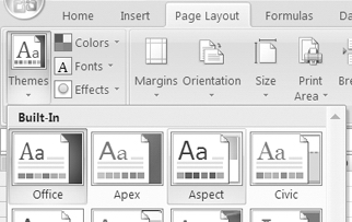
Figure 5-20. Themes gallery
- In your pivot table, the colors and fonts change to match the colors and fonts in the Aspect theme, as shown in the Aspect sample.
- Click the Aspect theme to select it, and your pivot table now has that theme's fonts and colors applied.
The Aspect theme uses the Verdana font for headings and body and darker colors. Because the Verdana font is wider than the Calibri font, your pivot table is wider. In the Themes group on the Page Layout tab, the icons have changed to reflect the colors, fonts, and effects of the current theme. In the PivotTable Styles gallery, the styles use the colors from the new theme.
Other features are also affected by the change in themes. The font in the row and column buttons changes to the Body font for the current theme. On Sheet1, where your data is stored, the table has changed, using the colors and fonts of the current theme. The Table style gallery also shows styles in the current theme.
- To reapply the Office theme, return to the Themes gallery, and click the Office theme.
Saving the File
You can save your file now as WorkOrders_03.xlsx. That will leave the original file unchanged since its last save, and you can use the new file for your work in the next chapter.
Summary
In this chapter, you added formatting to a pivot table to enhance the data presentation. With suitable formatting you can make pivot tables easier to read and highlight specific data. You also applied, modified, and created pivot table styles to make formatting consistent throughout your workbook. Finally, you examined themes and saw that they have an overriding impact on your pivot table formatting and on other features in the workbook.