
CHAPTER 7
Creating a Pivot Table
from External Data
So far, you've created pivot tables from data that is stored in Excel tables. You can also create a pivot table in Excel from many kinds of external data sources. In this chapter, you'll connect to data that is outside Excel, and you'll create pivot tables from that data. You can download and work with a text file, an OLAP cube, and a Microsoft Access query to see how the pivot table creation process is slightly different depending on the source data. You'll also see some differences in pivot tables that are created from external data sources compared to pivot tables based on Excel data.
To create a pivot table from data that is outside Excel, you can import the data to a worksheet and create the pivot table from the imported data, or you can create a connection to the external data, telling Excel where the file is and how to connect to it, and then create a pivot table from the data.
You'll use both techniques to create pivot tables in the examples in this chapter:
- First, you'll import data from a text file onto a worksheet. Instead of creating an Excel table from the data and using that as the source for your pivot table, you'll create a pivot table from the unformatted external data to show employee test results.
- Next, you'll connect to a query in an Access database and create a pivot table to show shipment information.
- Finally, you'll connect to an OLAP cube to summarize sales information from another database.
Creating a Pivot Table from a Text File
You have been sent a text file from the human resources (HR) department, and the HR manager has asked you to create a report from this file to summarize the employee test scores by location. Each month a new version of the text file will be created and sent to you so you can create an updated report. To make the updates easier, you'll connect to the text file and create a pivot table from the external data.
The first time you use a text file as the source for a pivot table, you should check it to make sure it's set up correctly. If necessary, you can make changes to the file so it's ready to use as the source for your pivot table. You'll download and check the sample file that contains the employee test scores.
- Download the text file named
EmployeeData.txt, and save it in one of your folders. In this example, the file was saved in thec:Datafolder. - Using Notepad or another text editor program, open the
EmployeeData.txtfile to see the data it contains (see Figure 7-1).
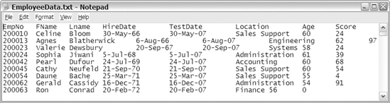
Figure 7-1. Text file opened in Notepad
- Identify the type of text file you have opened—delimited or fixed width. This is a delimited text file in which the field data in each row is separated by an identified character, or delimiter. In this file, the delimiter is the tab character, and in other files a comma or other character may be used. In a fixed-width text file, each field is a set number of characters, and there is no separator between the fields.
- Field headings are required in the first row of the text file if you plan to use it to create a pivot table. If the headings are missing, you should add them before using the file as the source for your pivot table. This file contains a heading row that identifies the fields in each record—EmpNo (employee number), FName, LName, HireDate, TestDate, Location, Age, and Score.
- Ensure that there is a line break at the end of each record to separate the records. In this file, each record starts on a new line.
- The text file looks fine, so close the text file without making any changes.
Importing the Text File
After you have examined the text file, the next step is to open the workbook in which you want the pivot table or create a new workbook where you will create the pivot table. To create the report for the HR manager, you'll create a new workbook and build the pivot table there using the EmployeeData.txt file.
As a first step, you'll import the text file onto a worksheet, and later you'll create the pivot table from the imported data:
- In Excel, create a new blank workbook.
- On the Ribbon, click the Data tab, and in the Get External Data group, click From Text (see Figure 7-2).
Note You may see a single Get External button instead of several buttons. Click the Get External Data button, and then click From Text.
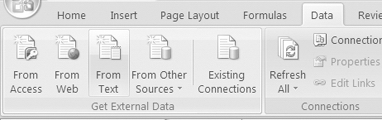
Figure 7-2. From Text command on the Ribbon
- In the Import Text File dialog box, select the folder in which you stored the
EmployeeData.txtfile, select the file, and click Import (see Figure 7-3).
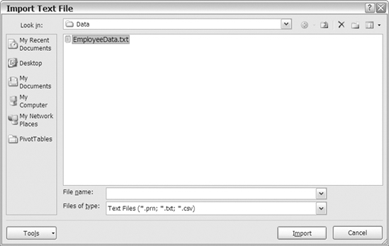
Figure 7-3. Import Text File dialog box
- On the Step 1 of 3 page of the Text Import Wizard, the wizard examines the file to determine which type of text file you are importing and shows a preview of the data. If it is incorrect, you can change the original data type. For the
EmployeeData.txtfile, select Delimited (see Figure 7-4).
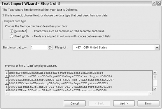
Figure 7-4. Text Import Wizard's Step 1 of 3 page
In the preview section at the bottom of the dialog box, you can see the first few rows of data from the text file with small squares between the fields. These represent the tab characters that separate the fields in the text file.
- The import is set to start at row 1, which is correct for this file. If a text file had a few rows at the start that you did not want to import, you could change the start row.
- The file origin shown in Figure 7-4 is 437: OEM United States, but this may be different on your screen depending on your regional settings in the Windows Control Panel. In most cases, you can leave this option at the default setting. However, if a text file is known to be from a different location and uses a character set, you can change the file origin.
- Click Next to go to Step 2.
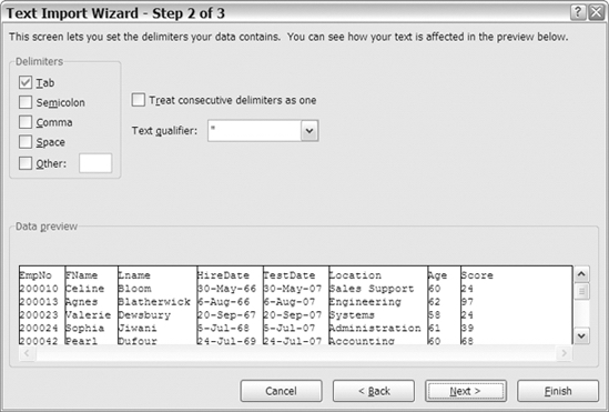
- On the Step 2 of 3 page of the Text Import Wizard, the wizard has applied a tab delimiter to the text and shows a preview of the separated data. If the file uses a different delimiter, such as a comma, you can change the delimiter. For the
EmployeeData.txtfile, select Tab (see Figure 7-5).
Figure 7-5. Text Import Wizard's Step 2 of 3 page
- Click Next to go to the next step.
- On the Step 3 of 3 page of the Text Import Wizard, you can adjust the data type for each column. In this example, General will be used for each column, and for other text files you can change the data type for one or more columns if required. To change a data type, click a column heading in the Data Preview area, and select a column data format for that column (see Figure 7-6).
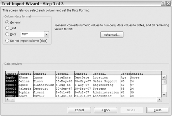
Figure 7-6. Text Import Wizard's Step 3 of 3 page
- Click Finish to close the Text Import Wizard.
- In the Import Data dialog box, leave the default setting for Existing Worksheet and the formula (=$A$1) that references cell A1, and click OK (see Figure 7-7).
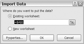
Figure 7-7. Import Data dialog box
- The data from the
EmployeeData.txtfile appears on the worksheet, and you can create a pivot table from this imported data. - Save the Excel file. In this example, the file was named
EmpDataPivot.xlsxand saved in thec:Datafolder.
Modifying the Connection
By importing the EmployeeData.txt file, you created a connection in the workbook. This is a link to the EmployeeData.txt file outside Excel, and you can change some settings for this connection to control how it works. For example, you can specify how often the data should be refreshed and what should happen to the formatting when the data is refreshed.
You'll view and test the current connection settings and then change some of the settings for the connection to the EmployeeData.txt file:
- Select a cell in the imported data.
- On the Ribbon, click the Data tab, and in the Connections group, click Properties (see Figure 7-8).
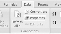
Figure 7-8. Properties command on the Ribbon
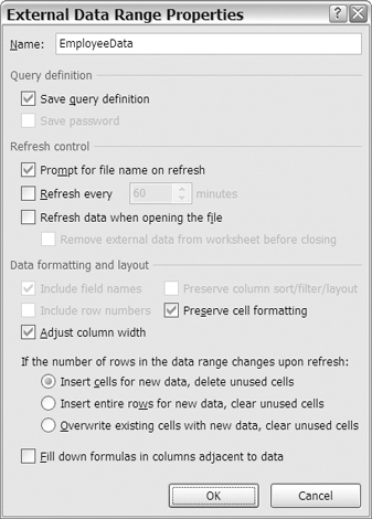
- The External Data Range Properties dialog box opens and shows the current settings for this connection, with the name of the external data range, EmployeeData, shown at the top of the dialog box (see Figure 7-9).
Figure 7-9. External Data Range Properties dialog box
- In the Refresh Control section of the dialog box, remove the check mark from Prompt for File Name on Refresh. With this setting turned on, you would have to select the
EmployeeData.txtfile each time you refreshed the data. This setting may be useful if the file name changes each day, for example, if there is a daily text file download. In this case, the text file will remain the same, so you won't want to be prompted during each refresh. - In the Refresh Control section of the dialog box, add a check mark to Refresh Data When Opening the File. With this setting turned on, you will ensure that the data is current in the Excel file. If there have been changes to the
EmployeeData.txtfile, the revised data will be available in the Excel file. - Click OK to close the External Data Range Properties dialog box.
You'll leave the Excel file open while you make a change in the EmployeeData.txt file, and then you'll refresh the external data in Excel to test the settings you changed. The first name in the text file was typed incorrectly, so you'll change it.
- Using Notepad or another text editor program, open the
EmployeeData.txtfile, and in the first record, change the name from Celine to Celina. - Save and close the
EmployeeData.txtfile. - In Excel, right-click a cell in the imported data.
- In the context menu, click Refresh.
- The external data is refreshed, and you were not prompted to select the
EmployeeData.txtfile. The name in the first record has changed to Celina.
Next, you'll close the Excel file and then make another change to the EmployeeData.txt file. When you reopen the Excel file, the external data should automatically refresh, because you changed that setting for the external data connection. The first employee's name needs further correction, so you'll make the additional change.
- In Excel, save and close the
EmpDataPivot.xlsxfile. - Using Notepad or another text editor program, open the
EmployeeData.txtfile, and in the first record, change the last name from Bloom to Blume. - Save and close the
EmployeeData.txtfile. - In Excel, open the
EmpDataPivot.xlsxfile, and check the name in the first record to verify that it was changed from Bloom to Blume.
Changing the Security Settings
If the name in the first record was not changed to Blume, your security settings may have prevented the update. You may be able to adjust these settings, as described in this section, or temporarily allow updates each time you open the file.
If the name in the first record was successfully changed, your security settings are allowing data connections and won't need to be changed. You can skip this section and proceed to the next section to create the pivot table.
- Below the Ribbon, you may see a security warning that tells you the data connections have been disabled (see Figure 7-10).

Figure 7-10. Security warning for data connections
- If the Security Warning bar is visible, click the Options button.
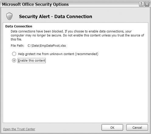
- In the Microsoft Office Security Options dialog box, read the information about the data connection and the file path for the Excel file. Because you know and trust the source data, select the Enable This Content option, and click OK (see Figure 7-11).
Figure 7-11. Microsoft Office Security Options dialog box
- The external data is refreshed, and the name in the first record has changed to Blume. The Security Warning bar disappeared from below the Ribbon. You have enabled the content temporarily, and the Security Warning bar may reappear if you close and reopen the Excel file.
If the Security Warning bar was not visible but the file did not refresh, your security settings may have the message bar turned off. The content from the external data file has been blocked, but you do not see the warning. You can manually refresh the external data:
- Right-click a cell in the Excel table, and in the context menu, click Refresh.
- If a Microsoft Office Excel Security Notice dialog box appears, read the information about the external data source. Because you know that this source can be trusted, click OK (see Figure 7-12).
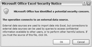
Figure 7-12. Microsoft Office Excel Security Notice dialog box
- The external data is refreshed, and the name in the first record has changed to Blume. You have enabled the connection temporarily, and the Security Notice dialog box may reappear if you close and reopen the Excel file and try to refresh the data.
To permanently allow the connection each time you open the Excel file, you can add the source data file to a trusted location. These are folders that you or your system administrator has designated as safe locations, and all files in these folders can be opened without a security warning. To view or change these locations or to change other security settings, you can use the Trust Center, accessible through the Microsoft Office Button (click Excel Options, and then click Trust Center). If you're not sure about these settings, check with your system administrator.
Creating the Pivot Table
Now that the text file has been imported to a worksheet, you can create a pivot table from the external data. The HR manager has asked for a summary of employee test scores by location, so you will show a list of locations with a count of employees and the average test score for each location.
Usually you would create an Excel table from the data on a worksheet and then use the Excel table as the source for the pivot table. However, this data is in an external range that has the name EmployeeData, which you saw in the External Data Range Properties dialog box. If you try to create an Excel table from this data, it will override the external data range, and you will lose your connection to the text file.
- Select a cell in the imported data.
- On the Ribbon, click the Insert tab, and in the Tables group, click PivotTable (see Figure 7-13).
Caution Use the PivotTable command. Do not click the Table command and create an Excel table, or you will remove your connection to the text file.
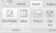
Figure 7-13. PivotTable command on the Ribbon
The Create PivotTable dialog box opens and shows the address of the external data range, Sheet1!$A$1:$H$501, in the Table/Range box. You can use the external data range address as the source range, and the pivot table will automatically adjust if rows are added or removed in the source data. However, using the name of the external data range may make the data source easier to identify when working with the pivot table.
- In the Table/Range box, type EmployeeData, which is the name of the external data range, and then click OK (see Figure 7-14).
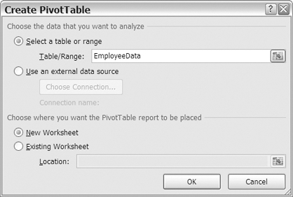
Figure 7-14. Entering the external data range name
- A new worksheet, Sheet4, is inserted with an empty pivot table. In the PivotTable Field List pane, you can see the field names from the
EmployeeData.txtfile. - In the PivotTable Field List pane, add a check mark to Location to add that field to the Row Labels area.
- In the PivotTable Field List pane, add a check mark to EmpNo to add that field to the Values area and then change the field so it is summarized by Count.
- In the PivotTable Field List pane, add a check mark to Score to add that field to the Values area and then change the field so it is summarized by Average. Change the number format for the score so it has no decimal places.
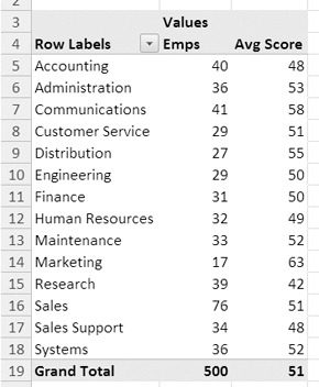
- To complete the pivot table, change the heading for Count of EmpNo to Emps, change Average of Score to Avg Score, and make the columns narrower (see Figure 7-15). These changes will make the report more visually appealing and easier for the HR manager to read. You can now send the report, showing the number of employees who were tested at each location and the average scores.
Note If the external data has changed, that will not be reflected in the pivot table until the imported data is refreshed and then the pivot table is refreshed. Refreshing the pivot table does not refresh the imported data.
Figure 7-15. Pivot table from text file
- Now that you have completed the pivot table, save and close the
EmpDataPivot.xlsxfile.
Creating a Pivot Table from an Access Query
Another source that you can use for pivot tables is a query in a Microsoft Access file. In this example, you'll download a small database in which shipments are recorded. You do not need a copy of Microsoft Access on your computer in order to connect to an Access database from Excel.
Connecting to the Access Query
Impressed by the report you created for the HR manager, the shipping manager has sent you a copy of the shipments database and has asked you to summarize the freight charges for each county. In the database is a query that combines data from three tables: Shipments, Contracts, and Counties. You'll connect to this query and create a pivot table to summarize the freight charges by county. When you create this report in Excel, employees who don't have Access installed will be able to view and manipulate the shipments report.
- Download the Access database file named
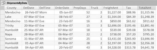
Shipments.accdb, and save it in one of your folders. In this example, the file was saved in thec:Datafolder. - The shipping manager has sent you a screen shot of the Access query named ShipmentsByDate, which is the query that you'll connect to when creating the pivot table (see Figure 7-16).
Figure 7-16. ShipmentsByDate query in Access database
- Before using this query for the first time, you'll confirm it contains all the fields you'll need for the pivot table. If anything is missing, you'll ask the shipping manager to make changes to the Access query. In the pivot table, you want to summarize the freight charges by county, and you can see that the County and FreightAmt columns are in the query results.
- You will also need the freight tax amounts in the pivot table totals, and that has been calculated in the query based on the county tax rate. The query also calculates the total amount, which is freight plus tax.
Tip It is best to include these line calculations in the Access query to ensure that the results are accurate, because the pivot table cannot calculate the line details.
- Now that you have verified that the query is set up correctly, you're ready to create the pivot table.
In the following steps, you'll create a new workbook and build the pivot table there using the query in the Shipments.accdb Access database. You'll connect to the query and create the pivot table directly from the data. Unlike the text file you used for the Employee test scores pivot table, you won't import the Access data onto a worksheet.
- In Excel, create a new blank workbook.
- On the Ribbon, click the Data tab, and in the Get External Data group, click From Access.
- In the Select Data Source dialog box, locate and select the
Shipments.accdbfile, and then click Open. - In the Select Table dialog box, select ShipmentsByDate, which is the query you want to use, and then click OK (see Figure 7-17).
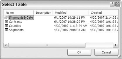
Figure 7-17. Select Table dialog box
- The Import Data dialog box opens, with a list of options for viewing the data. Select PivotTable Report from the list of view options, and select cell A1 on the existing worksheet as the location for the data (see Figure 7-18).
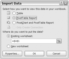
Figure 7-18. Import Data dialog box
- Click OK to close the Import Data dialog box.
An empty pivot table is created on Sheet1. In the PivotTable Field List pane, you can see the field names from the ShipmentsByDate query. You created a connection to the query in the Access database, and you can use its data in your pivot table.
You'll add fields to the pivot table layout to show a list of counties, with a count of shipments and the average total freight for each county:
- In the PivotTable Field List pane, add a check mark to County to add that field to the Row Labels area.
To count the shipments, you'll add the delivery date field, DelDate, to the Values area. Since each record has a delivery date, this will be a reliable field to use for the count.
- In the PivotTable Field List pane, add a check mark to DelDate, and then move that field to the Values area, where it will be summarized by count.
To calculate the average shipping cost, you'll add the total amount field, TotalAmt, to the Values area.
- In the PivotTable Field List pane, add a check mark to TotalAmt to add that field to the Values area, and then change the field so it is summarized by Average. Change the number format to Currency.
- To complete the pivot table, change the heading for Count of DelDate to Shipments, change Average of TotalAmt to Avg Total, and make the columns narrower (see Figure 7-19).
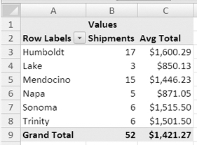
Figure 7-19. Pivot table from Access query
- Now that you have completed the pivot table for the shipping manager, save the file as
ShipmentPivot.xlsx. In this example, the file was saved in thec:Datafolder.
Modifying the Connection to the Access Query
By creating a pivot table from the Access query, you created a connection in the workbook. This is a link to the Access file outside Excel, and just as you did for the text file connection earlier, you can change some settings for this connection to control how it works.
You'll view the current connection settings and then change the settings for the connection to the ShipmentsByDate query to ensure that the data is refreshed frequently while the Excel file is open. Then, if the shipping manager opens your workbook first thing in the morning, the data will be refreshed throughout the day if the workbook is left open.
- On the Ribbon, click the Data tab, and in the Connections group, click Connections (see Figure 7-20).
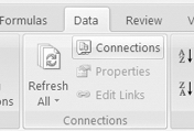
Figure 7-20. Connections command on the Ribbon
- The Workbook Connections dialog box opens and shows the connections in the active workbook. The Shipments connection is listed, and you can scroll to the right in the list to see the date and time that the connection was last refreshed (see Figure 7-21).
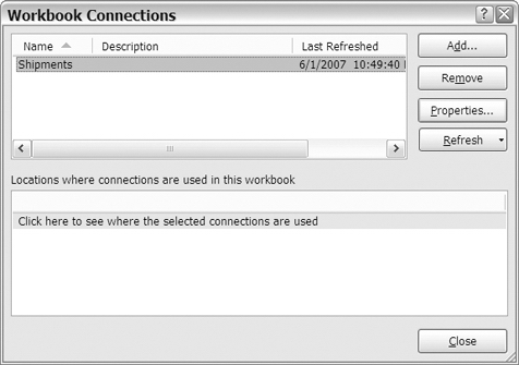
Figure 7-21. Workbook Connections dialog box
In the lower half of the Workbook Connections dialog box, you can view a list of locations where a connection is used in the workbook. You'll select the Shipments connection and see where it is used.
- Select the Shipments connection in the list at the top of the dialog box.
- In the lower section of the dialog box, point to the text that says Click Here to See Where the Selected Connections Are Used.
- When the text becomes underlined, click the underlined text, and you'll see the sheet, name, and location of the pivot table listed (see Figure 7-22).
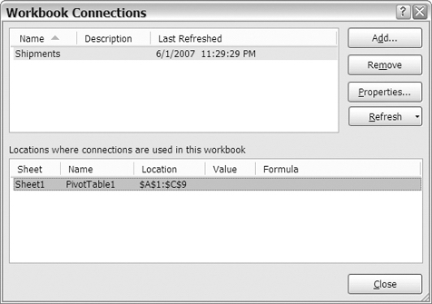
Figure 7-22. List of locations where the selected connection is used
When the list of locations is visible, you can use it to select any location that is listed. This feature is especially helpful if you have multiple connections and pivot tables in a workbook and want to understand how things were set up.
- Click the location information, and the pivot table on Sheet1 is selected.
From the Workbook Connections dialog box, you can access the Connection Properties dialog box to view or change the properties for the selected connection. You want to change the refresh settings for the connection, so you'll open the Connection Properties dialog box.
- With the Shipments connection selected in the list, click the Properties button. In the Connection Properties dialog box, on the Usage tab, you can see the date and time of the last refresh and the current settings for the connection. At the top of the dialog box are the connection name and description (see Figure 7-23).
Tip You can type a description to explain what data the connection contains, why the connection is used, or other notes that will help you when using the file.
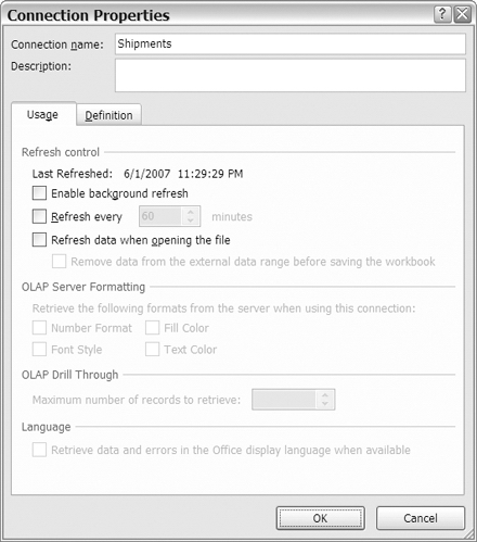
Figure 7-23. Connection Properties dialog box
- In the Refresh Control section, add a check mark to Refresh Every 60 Minutes, and change the time to 30 minutes. This will ensure that the external data is refreshed frequently, so if the data changes in the Access database, the revised information will be available in the Excel file.
Note This option is available only when using external data.
- Also add a check mark to Refresh Data When Opening the File. This will ensure that the external data is automatically refreshed as soon as the file opens.
- To see the settings that were stored when you created the connection, click the Definition tab (see Figure 7-24). You can see the connection type and the location of the connection file. The Connection String box contains information that tells Excel how to connect to the external data, and the Command Text box contains information about the Access query.
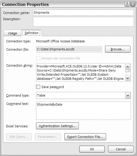
Figure 7-24. Definition tab in the Connection Properties dialog box
- Leave these settings untouched, and click OK to close the Connection Properties dialog box. Then click Close to close the Workbook Connections dialog box.
The Security Warning bar may appear, alerting you that the data connections have been disabled. Just as you did for the EmployeeData.txt file connection, you can click the Options button and enable the content. You can also add the source file to a Trusted Location to prevent the Security Warning bar from reappearing.
Using an Existing Connection to Create a Pivot Table
The shipping manager likes the pivot table you created to show the shipments per county and asks whether you can create another report in the same workbook. In this report, the number of shipments per delivery truck should be listed to see whether the loads are evenly distributed among the drivers.
After you have created a connection in a workbook, you can use it again to create a pivot table or to import data to a worksheet. You'll reuse the Shipments connection to create another pivot table. On Sheet2, you'll create a pivot table to summarize the data by truck to count the shipments per county for each delivery truck:
- Select Sheet2, where you'll create the new pivot table.
- On the Ribbon, click the Data tab, and in the Get External Data group, click Existing Connections (see Figure 7-25).
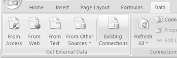
Figure 7-25. Existing Connections command on the Ribbon
Note If the active cell is in a pivot table, the Existing Connections command won't be available.
- In the Existing Connections dialog box, from the Show drop-down list, select Connections in this Workbook.
- In the list of connections, select Shipments, and click Open (see Figure 7-26).
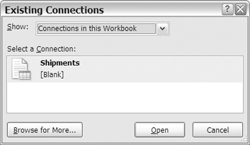
Figure 7-26. Existing Connections dialog box
- In the Import Data dialog box, select PivotTable Report as the way you want to view the data in your workbook. Leave the default settings for the Where Do You Want to Put the Data? option, and click OK.
- An empty pivot table is created on Sheet2. In the PivotTable Field List pane, you can see the field names from the ShipmentsByDate query.
Now you can create a different pivot table from the external data. You'll show a list of delivery trucks, with a count of shipments for each truck.
- In the PivotTable Field List pane, add a check mark to Truck, and then move that field to the Row Labels area.
- In the PivotTable Field List pane, add a check mark to DelDate, and then move that field to the Values area, where it will be summarized by Count.
- To complete the pivot table, change the heading for Count of DelDate to Shipments, change Row Labels to Truck, and make the columns narrower (see Figure 7-27).
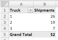
Figure 7-27. Reusing a connection to create another pivot table
- Now that you have completed the second pivot table, save the
ShipmentPivot.xlsxfile, and then close it.
Creating a Pivot Table from an OLAP Cube
Another source that you can use for pivot tables is an OLAP cube. This is aggregated data from an Online Analytic Processing (OLAP) database and can provide an efficient way for you to analyze data from SQL Server or another large database. In this example, you'll use a small OLAP cube, created from a hardware sales database. It will give you an opportunity to connect to the OLAP cube and see the differences in a pivot table that is created from this type of data source.
Understanding OLAP Cubes
Using a pivot table, you can easily connect to thousands of rows of data in an Excel table or in a data source outside Excel. However, for some applications, there may be hundreds of thousands or millions of rows of data, which could be more than a pivot table is able to process with acceptable speed or could exceed the memory limits of your computer. For example, a national hardware chain might have hundreds of thousands of purchases each month. To efficiently process and store that much data, large and powerful databases are required.
The vice president of sales has asked you to create a couple of reports from transaction data that has been collected by a hardware chain. Figure 7-28 shows a small sample of the data. For each transaction, information about the product, the selling location, the date, the quantity sold, and the price is entered.
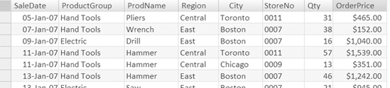
Figure 7-28. Hardware sales records
You won't be permitted to connect your pivot table directly to the transaction database. Instead, the database administrator will create a subset of the data for you in an OLAP cube. In the OLAP cube, instead of raw data, the data will be aggregated based on the information you need to analyze. In Excel, you can connect to the OLAP cube by creating a pivot table.
You send your report requirements to the database administrator so the OLAP cube can be created. The first report you'll create will show the total dollar amounts for each product group per region. The second report will show the quantity of each product sold, per year, for the East region.
To create the OLAP cube, the database administrator might use a product such as Microsoft SQL Server 2005 Analysis Services, Hyperion Essbase, Cognos PowerPlay, or Business Objects. In the OLAP cube, there are two types of data: measures and dimensions. The measures are numerical fields, such as quantity and price, that will be used in the Values area of a pivot table. The dimensions are the categories in which the data will be summarized, such as Region and ProductGroup. The dimensions are arranged in hierarchies of related fields. In the hardware sales data, Region, City, and StoreNo are in a hierarchy, as are ProductGroup and ProdName (see Figure 7-29). When the SaleDate field is added to the OLAP cube, a time hierarchy is automatically created, with Year, Quarter, Month, Week, and Day.
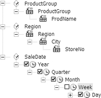
Figure 7-29. Dimensions in hierarchies
When you create a pivot table based on the OLAP cube, you'll see these hierarchies in the PivotTable Field List pane and in the pivot table layout. A pivot table that is based on an OLAP cube has some differences from a pivot table that is based on other data sources, and you'll see those as you create your hardware sales pivot table.
Connecting to an OLAP Cube
The database administrator e-mails to let you know that the OLAP cube is ready for you to use. The only way that the OLAP cube data is available in Excel is through a pivot table. You'll take advantage of that limitation and create a pivot table simply by opening the cube file in Excel. From the empty pivot table, you'll create your first report, showing the sales by product group and by region:
- Download the OLAP cube file named
HardwareSales.cub, and save it in one of your folders. In this example, the file was saved in thec:Datafolder. - In Excel, click the Microsoft Office Button, and click Open.
- In the Open dialog box, in the Files of type drop-down list, choose All Files (*.*).
- In the
c:Datafolder, select theHardwareSales.cubfile, and click Open. - If the Microsoft Office Excel Security Notice dialog box appears, click Enable to allow the data connection.
- The connection to the OLAP cube is created, an empty pivot table appears on the active worksheet, and the PivotTable Field List pane shows the fields from the OLAP cube (see Figure 7-30).
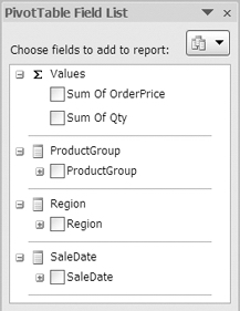
Figure 7-30. PivotTable Field List pane for OLAP cube fields
When the data source is an OLAP cube, the PivotTable Field List pane looks different than it does for other data sources. At the top is a list of Values, and these are the only fields that can be placed in the Values area. These are the measures, which are the numeric fields from the source data, and they can be placed only in the Values area. In the transaction database, OrderPrice is the total price for each order, and Qty is the quantity sold in each order.
Below Values in the PivotTable Field List pane are the remaining fields, and these can be placed in the Row Labels, Column Labels, or Report Filter area. These are the dimensions, and they look different than fields from other data sources because they have plus and minus buttons that show the fields in a hierarchy. For example, click the plus sign beside SaleDate, and the field expands to show Year, Quarter, Month, and Day.
The vice president of sales has asked for a report on the total sales for each product group in each region, so you'll add the ProductGroup, Region, and Sum Of OrderPrice fields to the pivot table layout:
- In the PivotTable Field List pane, add a check mark to ProductGroup, and then move that field to the Column Labels area.
- In the PivotTable Field List pane, add a check mark to Region, which will appear in the Row Labels area.
- In the PivotTable Field List pane, add a check mark to Sum Of OrderPrice, which will be added to the Values area, where it will be summarized by Sum.
Note The summary function cannot be changed for Values in a pivot table that is based on an OLAP cube.
- To complete the pivot table, format the values as currency with zero decimal places (see Figure 7-31).
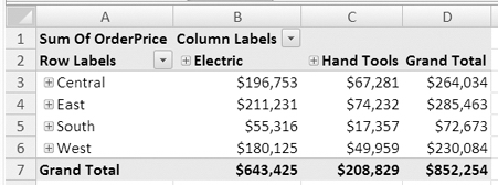
Figure 7-31. Pivot table based on an OLAP cube
- Now that you have completed the first report, save the file as
HardwarePivot.xlsx. In this example, the file was saved in thec:Datafolder.
Modifying the Connection to the OLAP Cube
By opening the OLAP cube file in Excel, you created a pivot table and a connection in the workbook. You'll view the current connection settings to see the settings that are available when an OLAP data source is used:
- On the Ribbon, click the Data tab, and in the Connections group, click Connections.
- In the Workbook Connections dialog box, select the HardwareSales connection, and click Properties.
- In the Connection Properties dialog box, you can see the date and time of the last refresh and the current settings for the connection. The Enable Background Refresh setting is not available, but the OLAP Server Formatting, OLAP Drill Through, and Language settings are available (see Figure 7-32).
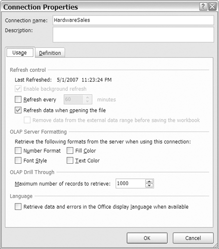
Figure 7-32. Connection Properties dialog box for OLAP-based pivot table
- Add a check mark to Refresh Data When Opening the File. This will ensure that the external data is refreshed as soon as the file opens. If the OLAP cube has been updated, you'll automatically be connected to the new data.
- Click OK to close the Connection Properties dialog box, and click Close in the Workbook Connections dialog box.
Next, you'll create your second report to show the quantity of each product sold, per year, for the East region. You want to limit the data to show only one region, so you'll move that field to the Report Filter area:
- Select a cell in the pivot table, and in the PivotTable Field List pane, move the Region field to the Report Filter area.
- Click the Region drop-down list in cell B1, and then click the + sign beside All to open the list of regions.
- Select East, which is the region you want in your report, and then click OK (see Figure 7-33).
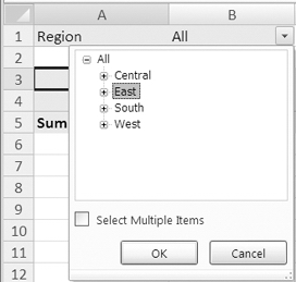
Figure 7-33. Report filter for East region
- In this report, you want to see the quantities sold, so in the PivotTable Field List pane, remove the check mark from Sum Of OrderPrice, and add a check mark to Sum of Qty.
Note For a pivot table based on an OLAP cube, the measures (numeric fields) can be added only to the Values area of the PivotTable Field List pane.
- In the PivotTable Field List pane, move the ProductGroup field to the Row Labels area.
For this report, you're interested in the individual products, so you'll expand the field so all the product names are visible.
- Select a cell that contains a ProductGroup label. For example, select cell A4, which contains the Electric label.
- On the Ribbon, under the PivotTable Tools tab, click the Options tab.
- In the Active Field group, click Expand Entire Field (see Figure 7-34).
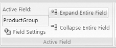
Figure 7-34. Expand Entire Field command
Tip Later, to hide the product names, you could select a ProductGroup label and then click the Collapse Entire Field command on the Ribbon.
The product names under each product group become visible, and you can see the total quantity for each product. Next, you'll add the SaleDate field to see the totals per year. Because the pivot table is based on an OLAP cube, you won't have to group the date field in order to see the totals per year. You'll examine the SaleDate field in the PivotTable Field List pane and then add it to the pivot table layout.
- In the PivotTable Field List pane, click the + sign to the left of the SaleDate field's check box. This will expand the hierarchy for SaleDate (see Figure 7-35).
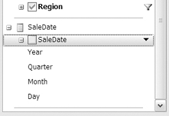
Figure 7-35. The expanded SaleDate hierarchy
- Add the SaleDate field to the Column Labels area. Because Year is the highest level in the SaleDate hierarchy, the Year labels, 2007 and 2008, appear in the Column Labels area (see Figure 7-36). The report now shows the total quantity sold per year for each product in the East region.
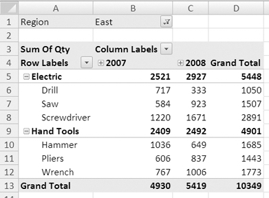
Figure 7-36. The completed pivot table
Tip To see the quantities sold per quarter, select one of the Year labels, and click the Expand Entire Field command on the Ribbon. To hide the quarters, click the Collapse Entire Field command.
- Now that you have completed the pivot table, save and close the
HardwarePivot.xlsxfile
Summary
In this chapter, you created connections to data outside Excel, and you created pivot tables from that data. With this capability, you can reach beyond your Excel data and report on data that is stored in other formats.
To work with a text file, you imported the data to a worksheet and created a pivot table from the imported data. You changed the data in the text file and refreshed the pivot table to show the updated data. If necessary, you changed the security settings to allow the connection to the external data.
Next, you connected to a query in an Access database and built a pivot table from that data. Then you modified the connection to ensure that the data was refreshed frequently. You used the features in the Workbook Connections dialog box to list the locations where the selected connection was used and to go to that location. In the same workbook, you created a second pivot table, based on the existing connection.
Finally, you connected to an OLAP cube by simply opening the cube in Excel. This automatically created a connection to the OLAP cube and an empty pivot table. While working on this pivot table, you saw differences in the fields in the PivotTable Field List pane and collapsed and expanded the fields in the pivot table.