Chapter 5 Data Transformation

Introduction

Zipf’s Law

Term-By-Document Matrix

Text Filter Node

Frequency Weightings

Term Weightings

Filtering Documents

Concept Links

Summary

References

Introduction

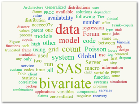
You saw in Chapter 4 that the first task of text mining analysis is to break down the text into a bag of words or tokens. Then, you apply various linguistic rules to identify the parts of speech, synonyms, noun groups, attributes, etc. Even before doing this exercise, a good understanding of what is being talked about in a corpus can be obtained by looking at the counts of the words extracted from the corpus. A current popular technique to visually represent prominent terms in text is using a word cloud or text cloud. This is an easy and visually appealing way of presenting the frequency of words in text as a weighted list. The font size of the words represents the frequency of the word. High frequency words appear in a bigger font size. There are various online resources available for free that can be used to generate a word cloud. Display 5.1 shows a word cloud for text from five random SAS Global Forum papers from our SAS Global Forum corpus. It is clearly evident that the terms “data,” “SAS,” and “bivariate” appear frequently in this corpus.

Display 5.1: Word Cloud

Source: http://worditout.com

Zipf’s Law

`

The most widely celebrated theory on the distribution of words in a large corpus is given by George Zipf, popularly known as Zipf’s law. This law was first stated by Estoup (1916), and later popularized by Zipf (1949). Manning and Schutze (1996) evaluate Zipf’s law using Mark Twain’s Tom Sawyer. According to Zipf’s law, if you rank order the frequency of occurrence of the words in a corpus, you can observe an approximate mathematical relationship between the position of the word (or the rank) and the frequency of occurrence of the word, as stated below:

$\mathit{f}\propto \frac{1}{\mathit{r}}\mathit{o}\mathit{r}\mathit{f}.\mathit{r}=\mathit{k}$ (Equation 5.1)

In this equation, f is the frequency of occurrence of the word, r is the rank of the word, and k is a constant.

Zipf’s law was widely applied to study different types of human behavior. In many cases, it was observed that the law holds true only for small corpora within processing capabilities during that time. When this law was applied to the SAS Global Forum corpus, we saw a big deviation in the constant term (frequency*rank) as shown in Table 5.1.

Table 5.1: Applying Zipf’s Law to SAS Global Forum Papers

Term	Frequency	Rank	Frequency*Rank
+ be	77920	1	77920
+ sas institute	42292	2	84584
+ data	42224	3	126672
+ use	25155	4	100620
+ variable	15218	5	76090
--------------
+ method	4009	87	348783
+ add	3991	88	351208
+ order	3931	89	349859
+ test	3905	90	351450
+ specify	3833	91	348803
--------------
+ complex filter	3	19926	59778
+ opportunity cost	3	19928	59784
data lineage	3	19929	59787
auditability	3	19930	59790
monolithic	3	19931	59793

However, Zipf’s law continues to generate interest even today. It is universally accepted that Zipf’s law gives a rough distribution of the frequency of words in a corpus. You can always identify a small set of words that account for almost 50% of the words in the corpus and identify a large set of words that occur very infrequently. You will find that these rare words account for a considerable portion of the text. The law tends to explain two forces that are controlled by the speaker and the hearer. The speaker is trying to minimize his effort by using fewer different types of words most often, and the hearer is trying to minimize his effort by having a large number of rare words (Marie, 1992).

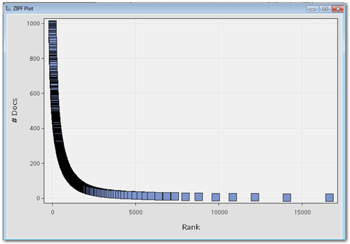
Instead of term frequency, SAS Text Miner uses the frequency of number of documents for a word to rank order the terms. Display 5.2 shows the ZIPF plot from the Text Filter node results for the SAS Global Forum corpus.

Display 5.2: ZIPF Plot from Text Filter Node Results

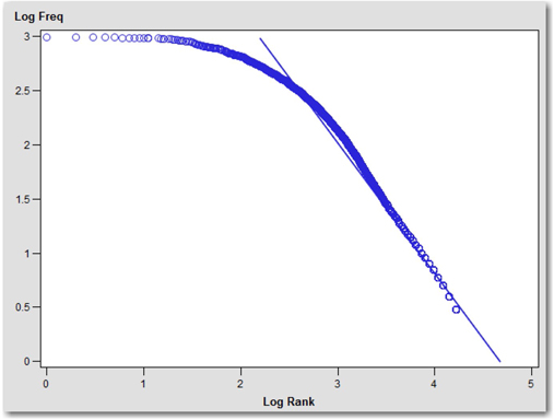
Mandelbrot (1954) has extensively validated Zipf’s law. He identified that the law holds true only in a restricted range of the word distribution. He noted that the distribution according to the law is a bad fit, especially for high and low rank terms. Zipf’s law belongs to the class of power laws (y = kx^c), with c=-1. According to a power law, the plot of frequency of the word and rank of the word on a logarithmic scale is approximately linear with slope -1. Display 5.3 shows the plot of frequency of the word and the rank on a logarithmic scale. You can clearly see a huge deviation from linear distribution for very high ranks. To achieve a better fit, Mandelbrot modified Zipf’s law and suggested the relationship between rank and frequency as the following:

f = P(r + ρ)^-B or log f = log P - B log(r + ρ) (Equation 5.2)

In this equation, P, B and ρ are parameters of the text. For B=1 and ρ = 0, Mandelbrot’s formula simplifies to Zipf’s law.

Display 5.3: Term Frequency versus Term Rank (Log Scale)

Term-By-Document Matrix

The fundamental idea of applying classical data mining techniques to text mining relies on transforming text data (unstructured) to numbers (structured). This numerical representation of the text takes the form of a spreadsheet-like structure called a term-by-document matrix. In this matrix, dimensions are determined by the number of documents and number of terms in the corpus. Here is the same example from Chapter 1 for a term-by-document matrix.

Consider a collection of three reviews (documents) of a book as provided below.

Document 1: I am an avid fan of this sport book. I love this book.
Document 2: This book is a must for athletes and sportsmen.
Document 3: This book tells how to command the sport.

Parsing this document collection generates the following term-by-document matrix in Table 5.2.

Table 5.2: Term-By-Document Matrix

Term/Document	Document 1	Document 2	Document 3
I	2	0	0
am	1	0	0
an	1	0	0
avid	1	0	0
fan	1	0	0
of	1	0	0
this	2	1	1
book	2	1	1
love	1	0	0
is	0	1	0
a	0	1	0
must	0	1	0
for	0	1	0
athletes	0	1	0
and	0	1	0
sportsmen	0	1	0
tells	0	0	1
how	0	0	1
to	0	0	1
command	0	0	1
the	0	0	1
sport	1	0	1

There are many theories that discuss what numbers should go into the cells of this matrix. In the simplest approach, each cell of the term-by-document matrix is allowed to contain the term frequency or the number of times a term appears in the document (as shown in Table 5.2). Another simple measure is the presence or absence of a term in a document. A detailed discussion about term weighting techniques appears in the next section. Once you have a table-like structure, traditional statistical methods can be comfortably applied to identify key inputs (terms) that differentiate or categorize the documents without having to use any grammar rules. Table 5.2 can be visualized as rows identified by documents and columns identified by terms. Even with a decent size corpus of a thousand documents, you can end up with thousands of unique terms, resulting in a huge dimensional matrix. The size of a term-by-document matrix can grow exponentially with more documents and more terms being extracted. As you can see from Table 5.2, there are many zeros in this table. This is because the rare words make up a significant portion of the text. Sparseness is a key characteristic of a term-by-document matrix compared to any typical table used for data mining. This is in-line with what is expected according to Zipf’s law. The other two features of this table that make it unique are the absence of non-negative values and missing values. Algorithms that process text data have been developed to comply with the properties of a term-by-document matrix: sparseness, non-negative values, and high dimensions.

Text Filter Node

In SAS Text Miner, the Text Filter node is primarily used for filtering documents and configuring the term weight and frequency weight settings. An important objective of text mining analysis is to differentiate the documents in the corpus. In this effort, the key task is to identify significant terms that can discriminate the documents. Research in the field of information retrieval has shown that using simple term frequencies does not help in document discrimination. Terms with low and high overall frequencies are found to be very bad discriminators. The best discriminators are those with neither too high nor too low frequencies–with document frequencies between n/10 and n/100 for a corpus of n documents.

Various techniques are available that use term frequency, document frequency, number of documents that the term occurs in, and the size of the corpus to derive a weight for each term. Terms that occur very often in a document are assigned a higher weight and are considered important because they better describe the document. Terms that occur less frequently in the corpus are assigned a higher weight because they better discriminate the documents in the corpus. The value that goes into the term-by-document matrix is calculated using these weights. Two different types of weights are used. The first one is frequency weight, also called the local weight (within a document). Frequency weighting is the transformation of the frequency of the occurrence of the term in a document using a weighting function. The other one is term weight, also called global weight (corpus wide). A term weight is assigned to the term based on the overall frequency and document frequency. The cell value in a term-by-document matrix is a weighted frequency value derived by multiplying the local weight and the global weight. One of the most popular weighting schemes in the field of information retrieval is tf-idf (term frequency, inverse document frequency) (Salton and Buckley, 1988). The term frequency (tf) (or the local measure) is calculated with the following equation:

$$\mathit{t}\mathit{f}=\frac{\mathit{t}\mathit{d}\mathit{f}}{\text{max }\mathit{t}\mathit{d}\mathit{f}}$$

In this equation, tdf is the document-specific frequency for a term, and max tdf is the frequency of the most frequent term in a document. Longer documents tend to have more terms (and, hence, a high tdf). These high frequencies are normalized using max tdf. The idf (Sparck Jones, 1972) portion of the weighting scheme is the global frequency measure, which is calculated with the following equation:

$$\mathit{i}\mathit{d}\mathit{f}=\mathit{log}\left(\frac{\mathit{N}}{\mathit{d}{\mathit{f}}_{\mathit{t}}}\right)$$

In this equation, N is the size of the collection, and df_t is the number of documents in which the term t appears. The tf-idf measure is simply the product of the local weight and global weight. The following section discusses different weighting schemes available in SAS Text Miner.

Let f_ij be the raw frequency of ith term in the jth document. You first use a function g(.) to transform the raw frequency, g(f_ij). Let w_i be the weight of the ith term. The weighted frequency of the ith term for the jth document in a term-by-document matrix is given by g(f_ij)* w_i.

Frequency Weightings

SAS uses three different local frequency weighting property settings: log, binary, and none.

Log: g(f_ij) = log(f_ij + 1)

This is the default setting for this property and is used to control the effect of high frequency terms in a document.

Binary: g(f_ij) = 1

This is the equation if a term is present in a document. g(f_ij) = 0 is the equation if a term is absent in a document. This setting clearly doesn’t differentiate between documents where a term is heavily present and between documents where a term rarely occurs.

None: g(f_ij) = f_ij

With this setting, the raw frequency value is used as is with no transformation done. This does not mean that no frequency weighting method is used.

Term Weightings

With thousands of terms extracted from each document, the key question is, “Are all the terms in a document important?” Frequency weights help only in understanding the composition of a document. They do not help in identifying the terms that discriminate the documents. Each term is assigned a weight using any of the three different methods available in SAS. The fundamental assumption in assigning a weight to a term is that the term occurs in only a few documents, but it occurs many times in those few documents, and the term is significant in discriminating the documents. The three global frequency weighting methods available in SAS for assigning a weight to a term are entropy, mutual information, and inverse document frequency.

Entropy

Entropy is a sophisticated metric derived from the concept of information gain in the field of information theory developed by Claude Shannon in the 1940s. Shannon used the concept of entropy from statistics to solve the problems of maximizing information transmission over imperfect channels of communication. In statistical parlance, entropy measures the average uncertainty in a single random variable, X, and is usually denoted as the following:

$$-{\displaystyle \sum \mathit{p}(\mathit{x}){\log }_2}\mathit{p}(\mathit{x})$$

In this equation, p(x) is the probability that the random variable X takes the value of x. In text mining, this technique uses the random variable (which represents the distribution of words across the corpus) in the calculation of the weight for a term.

With the entropy method, the weight for term w_i is calculated using the following equation:

${\mathit{w}}_{\mathit{i}}=\mathbf{1}+{\displaystyle \sum {}_{\mathit{j}=1}^{\mathit{n}}}\frac{({\mathit{f}}_{\mathit{i}\mathit{j}}/{\mathit{g}}_{\mathit{i}}).{\mathit{log}}_2({\mathit{f}}_{\mathit{i}\mathit{j}}/{\mathit{g}}_{\mathit{i}})}{{\mathit{log}}_2(\mathit{n})}$ (Equation 5.3)

Here, g_i is the number of times that term i appears in the document collection, and n is the number of documents in the collection. Because the logarithms of zero are undefined, the product in the numerator of the formula is 0, if f_ij=0.

Entropy weight for a term is zero if the term appears exactly once in all of the documents.

${\mathit{w}}_{\mathit{i}}=1+{\displaystyle \sum {}_{\mathit{j}=1}^{\mathit{n}}}\frac{(1/\mathit{n}).{\mathit{log}}_2(1/\mathit{n})}{{\mathit{log}}_2(\mathit{n})}=1+\frac{\mathit{n}*\frac{1}{\mathit{n}}*(-{\mathit{log}}_2(\mathit{n}))}{({\mathit{log}}_2\mathit{n})}=1-1=0$

Entropy weight for a term is 1 if the term appears only once in onedocument.

${\mathit{w}}_{\mathit{i}}=1+{\displaystyle \sum {}_{\mathit{j}=1}^{\mathit{n}}}\frac{(1/1).{\mathit{log}}_2(1/1)}{{\mathit{log}}_2(\mathit{n})}=1+\frac{1*0}{\left({\mathit{log}}_2\mathit{n}\right)}=1$

For all other occurrences, the terms have a value between 0 and 1. Generally speaking, the terms that occur infrequently in a few documents get higher weights, meaning these terms are considered to be providing more information than terms with lower weights.

Inverse Document Frequency (IDF)

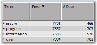
It is essential to study the relevance of collection frequency and document frequency in identifying important terms. For example, it is obvious that the SAS Global Forum corpus is dominated by terms such as “sas institute,” “paper,” “data,” and “information,” which are present in all the documents. These terms definitely do not help discriminate the documents. As shown in Display 5.4, the terms “macro” and “information” occur with approximately the same frequency (collection frequency) in the SAS Global Forum corpus, whereas the document frequency is considerably different for the two terms. Hence, it makes more sense to use document frequency instead of collection frequency in calculating the scaling factor.

Display 5.4: Term and Document Frequencies for the Terms “macro” and “information”

IDF is another measure used as a scaling factor in assigning an importance weight to a term. As the name implies, IDF calculates importance as the inverse of the frequency of occurrence of a term in documents. A term that appears infrequently is considered more important and is given a higher score, whereas a term with a high frequency of appearance is considered less important and is given a lower score.

${\mathit{w}}_{\mathit{i}}={\mathit{log}}_{\mathbf{2}}(\frac{\mathit{n}}{\mathit{d}{\mathit{f}}_{\mathit{i}}})+\mathbf{1}$ (Equation 5.4)

In this equation, df_i is the document frequency or the number of documents that contain the ith term. n is the number of documents in the collection.

If a term appears in every document, then the IDF weight for that term is the following:

${\mathit{w}}_{\mathit{i}}={\mathit{log}}_{\mathbf{2}}(\frac{\mathit{n}}{\mathit{n}})+\mathbf{1}=0+1=1$

The maximum IDF weight for a term occurs when the term appears in exactly one document. However, no upper limit exists for the maximum IDF weight because it depends on the number of documents and is equal to 1+log₂n.

An IDF weight value of zero indicates that the word appears in all documents and has an insignificant effect on discriminating the documents.

Mutual Information

Mutual information can be derived as the difference between the entropy of variable X and the entropy of variable X with the condition that X knows Y. That is, the mutual information is the reduction in uncertainty of X due to the knowledge of variable Y. In statistical parlance, mutual information between two variables works out to a symmetric non-negative measure of commonality between two variables. In text mining, this can be thought of as a measure of how much the presence of one term in a document tells us about whether the document belongs to a particular category. In SAS Text Miner, using this metric requires that your data contain a categorical target variable. In text mining problems where you have both structured and unstructured data, you will likely see a need for this metric because in most situations, you will have a target variable. This metric is defined as the following:

${\mathit{w}}_{\mathit{i}}={\mathit{max}}_{{\mathit{C}}_{\mathit{k}}}\left[\mathit{log}(\frac{\mathit{P}({\mathit{t}}_{\mathit{i}},{\mathit{C}}_{\mathit{k}})}{\mathit{P}({\mathit{t}}_{\mathit{i}})\mathit{P}({\mathit{C}}_{\mathit{k}})})\right]$ (Equation 5.5)

In this equation, P(t_i) is the proportion of documents that contain the term t_i. P(C_k) is the proportion of documents that belong to category C_k. P(t_i, C_k) is the proportion of documents that contain the term t_i and belong to category C_k. log(.) is 0 if P(t_i, C_k) = 0 or P(C_k) = 0.

The weight is proportional to the similarity of the distribution of documents that contain the term to the distribution of documents that are contained in the respective category. That is, in general, a higher mutual information weight for a term implies that the term tends to occur more in documents with the same target category. We demonstrate the benefits of this technique in Case Study 2.

None

With this setting, no term weight is applied (w_i = 1).

Term weights are used to scale the frequency weighting for a term in a document. Although the basic purpose of the previous methods is the same, it is difficult to make a definitive statement about which weight is the best metric. In general, entropy and IDF are most widely used in text mining applications, with entropy being more effective for smaller documents and IDF for larger documents. In practice, you are advised to try all of the methods and compare the results. Display 5.5 shows the property settings for term weightings from the Text Filter node Properties panel.

Display 5.5: Text Filter Node Properties Panel

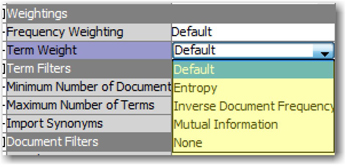
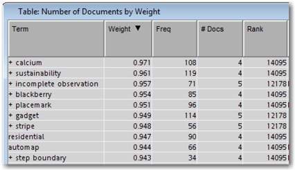
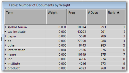
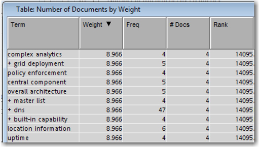
As the default setting, Entropy is used for the Term Weight property. In the presence of a categorical target, Mutual Information is used as the default setting. Let’s explore the effect of these settings on the SAS Global Forum corpus. Display 5.6 shows the top 10 terms based on term weight. Display 5.7 shows the top 10 terms based on rank. Clearly, the terms that have the largest weights are those that occur in very few documents. The terms that have the lowest ranks have low weights due to their high frequencies. This is essentially what is expected because terms like “sas institute,” “paper,” and “global forum” occur in every document and, hence, are not good differentiators.

Display 5.6: Top 10 Largest Weighted Terms

Display 5.7: Top 10 Highest Ranked Terms

Display 5.8 shows the top 10 terms as ranked by IDF. This is a completely different list when compared with the top terms from the entropy weight setting. All terms that appear in the same number of documents get the same weight.

Display 5.8: Top 10 Terms Based on IDF

Filtering Documents

Interactive Filter Viewer

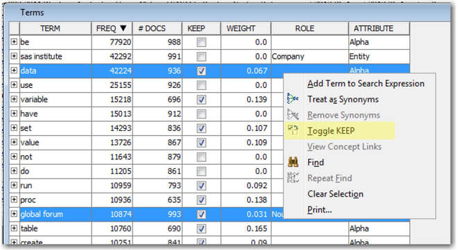
The interactive filter viewer is a handy feature of the Text Filter node to refine the results from parsing and filtering. You have seen the utility of this tool in Chapter 4for creating a custom synonym list using the parsed terms. You have studied various strategies during text parsing to filter irrelevant terms to lessen the number of terms used in post-parsing text mining tasks. After applying all of these techniques, you can encounter useless terms being retained and important terms being dropped in the list of filtered terms. Using the interactive filter viewer, you can browse through all of the parsed terms and manually modify the list by dropping or keeping terms. This is the most time-consuming step in the text mining process flow. The results of the text mining analysis are very sensitive to the terms that are included in the analysis. Hence, it is essential to invest time and effort in refining the list of selected terms manually by using the interactive filter viewer.

Display 5.9 shows the Terms table of the interactive filter viewer. The KEEP column in this table indicates whether a term is used or dropped from analysis. A checked box indicates an included term. To exclude the terms “data” and “global forum” from analysis, highlight the terms, right-click, and select Toggle KEEP (or you can directly clear the check box).

Display 5.9: Terms Table from the Interactive Filter Viewer

When you close the interactive filter viewer, you can save your changes, and the modified data is used in further analysis. An easy way to omit low-frequency words is by using the Minimum Number of Documents property setting. To exclude all of the terms that occur in less than 10 documents, enter a value of 10 for this property. The other property that can be used to control the number of terms is Maximum Number of Terms. Using this property, you can set a maximum limit on the total number of terms that are kept in the analysis based on their frequency. These different types of filtering properties come in very handy in reducing the noise from the data.

Document Search and Retrieval

In many situations when refining the terms and making a decision to include or exclude a term, you might want to quickly see the documents that contain that term. The interactive filter viewer contains a feature to search for documents in the corpus based on search expressions. A search expression can be a single term or a list of terms. Documents that match at least one of the terms are returned. The search results contain a relevance score for each document that indicates how well each document matches the search expression.

The matching documents are retrieved using the vector space model, which is the fundamental technique used in many information retrieval operations. In this model, all documents and search expressions are represented as vectors in the term space. The vector components are defined by the term weights given to the terms in the document. A similarity measure between two documents, d1 and d2, is calculated using the dot product (or cosine similarity) of the two vectors, V1 and V2.

similarity (d1, d2) = $\frac{{\mathit{V}}_1.{\mathit{V}}_2}{\left|{\mathit{V}}_1\right|\left|{\mathit{V}}_2\right|}$ (Equation 5.6)

The numerator in the equation represents the dot product between the two vectors. The denominator accounts for the various sizes of the documents by considering the Euclidean length of the document defined as the following:

$\left|{\mathit{V}}_{\mathit{i}}\right|=\sqrt{{\displaystyle \sum {\mathit{V}}_{\mathit{i}}^2}}$

Consider the following unit vector:

$${\mathit{v}}_{\mathit{i}}=\frac{{\mathit{V}}_{\mathit{i}}}{\left|{\mathit{V}}_{\mathit{i}}\right|}$$

Equation 5.6 can be rewritten as the following:

similarity (d1, d2) = υ₁ . υ₂ (Equation 5.7)

The search expression, in itself, is considered a short document. Term weights are calculated (also known as tf-idf weights) treating the search expression as a whole corpus. The tf-idf weight is the multiplication of term frequency and inverse document frequency. It has the following characteristics:

1. The value of tf-idf is highest when the term occurs many times within a fewer number of documents (i.e., higher discriminatory ability).

2. The value of tf-idf is lowest when the term occurs in almost all documents (i.e., lower discriminatory ability).

Consider an example corpus with just two documents.

Document 1: A vector space model uses a dot product to calculate similarity. This model defines vectors in the term space.

Document 2: A giant model of a spacecraft is being built for a movie based on space.

Consider the search expression (or query) “vector space model” used to retrieve matching documents from the corpus. Let inverse document frequency be used as the technique to calculate term weights in the corpus. Sample weights for the terms in the query are calculated using frequency. Table 5.3 shows the common words and one non-common word, “movie,” between the query and the documents.

Table 5.3: Weights for Words in the Sample Documents and Search Expression

Term	Search Expression			Document 1			Document 2
	Term Freq	Weight	Term Freq	Doc Freq	TF*IDF	Term Freq	Doc Freq	TF*IDF
vector	1	0.4	2	1	4	0	1	0
space	1	0.4	2	2	2	2	2	2
model	1	0.4	2	2	2	1	2	1
movie	0	0	0	1	0	1	1	2

Similarity between the search expression (Q) and document 1 (Doc1) is calculated using equation 5.7.

  Score (Q, Doc1) = (0.4 x 4) + (0.4 x 2) + (0.4 x 2) + (0 x 0) = 3.2

Similarly, the score between the search expression (Q) and document 2 (Doc2) is calculated.

  Score (Q, Doc2) = (0.4 x 0) + (0.4 x 2) + (0.4 x 1) + (0 x 2) = 1.2

We can conclude that document 1 is a better match with the query.

In this example, the inverse document frequency method is used for calculating term weights. SAS Text Miner uses a different weighting scheme that is not configurable. A relevance measure, between 0 and 1, for every document searched with the search expression is calculated. A value of 1 indicates a best match in the collection.

In the interactive filter viewer, you can enhance the search using the following techniques:

• +term returns only documents that include the term.

• -term returns only documents that do not include the term.

• +term1 term2 returns documents that include term1 and documents that include both term1 and term2. (Documents that contain term2 but not term1 are not returned.)

• +term1 +term2 returns only documents that include both term1 and term2.

• “text string” returns only documents that include the quoted text.

• string1*string2 returns only documents that include a term that begins with string1, ends with string2, and has text in between.

• >#term returns only documents that include the term or any of the synonyms that have been assigned to the term.

For example, to retrieve documents that contain the term “calcium” in the SAS Global Forum corpus, enter the term “calcium” or “+calcium” or “>#calcium” in the search expression. Or, you can locate the term “calcium” in the Terms table, right-click the term, and select Add Term to Search Expression. Display 5.10 shows the search results for the search expression “>#calcium.”

Display 5.10: Search Results for the Search Expression “>#calcium”

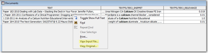
Out of the four results in Display 5.10, the RELEVANCE column shows that one of the documents from the search results is a best match with a score of 1. The other documents have a very low score. This is very clear if you look at the title of the paper:

• An Analysis of a Calcium Nutrition Educational Intervention for Middle School Students in Las Vegas, Nevada Using SAS^®

• Confessions of a Clinical Programmer: Dragging and Dropping Means Never Having to Say You’re Sorry When Creating SDTM Domains

• Dealing with Lab Data – Stacking the Deck in Your Favor

• The Next Generation: SAS/STAT^®

The first paper in the list, which got the best match score, refers and talks about calcium a lot. In the other three papers, the term “calcium” is referred to only occasionally and in examples. The relevance score is a useful measure in identifying irrelevant documents and excluding those documents from analysis.

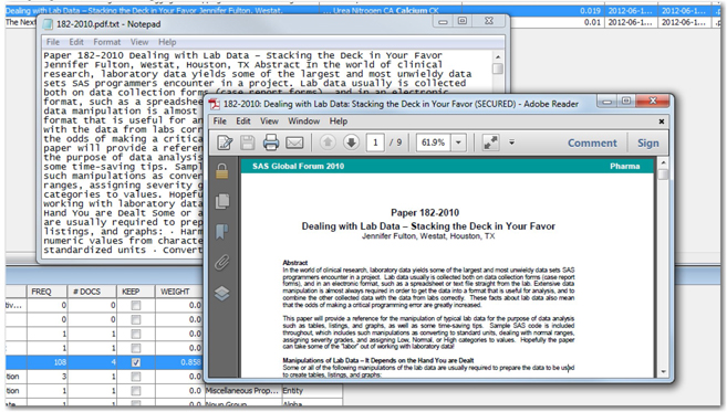
To read the full contents of the cell, right-click on the results, and select Toggle Show Full Text. In our example, because the text variable does not contain the full text and is being referred to in the actual SAS Global Forum papers using the paths to the files, you can access the full paper by right-clicking and selecting View Input File. Selecting View Original allows you to access the source file whose path is recorded in the variable with the role Text Location. Display 5.11 shows the two windows, with a .txt file and a .pdf file, that pop up when you select View Input File and View Original for one of the documents from the documents table.

Display 5.11: Viewing Source Documents from the Interactive Filter Viewer

Concept Links

Concept links help in understanding the relationships between words based on the co-occurrence of words in the documents. You can identify and define concepts in the text by selecting a keyword and exploring the words that are associated with this keyword using concept links. Concept links are intuitive and easy to understand because they are presented as interactive graphs. In the graph, the selected term is connected to other highly associated terms with a hub-and-spoke structure. The connected term can be expanded to display the terms associated with it. The structure can resemble a social network in which we can define multi-order associations. The width of the line between the center term and a concept link represents how closely the terms are associated. A thicker line indicates a closer association. The strength of association is calculated using binomial distribution. Here is the formula for calculating the strength measure as explained in the SAS Text Miner: Reference Help.

The strength of association between two terms, A and B in a corpus of r documents, is calculated as follows:

Strength = log_e(1/Prob_k)

Prob_k $={\displaystyle \sum {}_{\mathit{r}=\mathit{k}}^{\mathit{r}=\mathit{n}}[\mathit{n}!/[\mathit{r}!(\mathit{n}-\mathit{r})!]].{\mathit{p}}^{\mathit{r}}{(1-\mathit{p})}^{(\mathit{n}-\mathit{r})}}$

In this formula, n is the number of documents that contain term B.

k is the number of documents that contain both term A and term B.

p=k/n is the probability that term A and term B co-occur, assuming that they are independent of each other.

Concept links can be generated by right-clicking a term in the Terms tables in the interactive filter viewer, and selecting View Concept Links. Display 5.12 shows an example of the concept links for the term “calcium” from our example corpus.

Display 5.12: Concept Links for the Term “calcium”

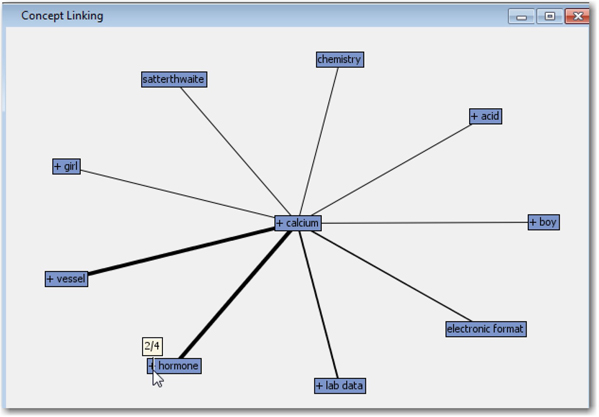
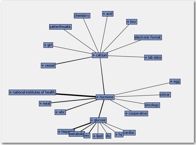
The term “calcium” is more strongly associated with the terms “vessel” and “hormone” than with the other words. If you hover over any term in the graph, you can see two numbers separated by a slash. The first number represents the number of documents in which the two terms co-occur, and the second number represents the total number of documents in which the specific term (“calcium”) occurs. You can right-click on any child term, and select Expand Links to display the terms associated with the child term. Display 5.13 shows the expanded version of the graph in Display 5.12. In the context of text mining customer feedback, an organization can easily identify the good or bad words that are associated with the products being reviewed. Concept links is a great feature to investigate the relationships between words in the corpus.

Display 5.13: Expanded Concept Links for the Term “calcium”

Summary

In this chapter, we discussed the transformation methods available in the Text Filter node that can be applied to a term-by-document matrix. You should experiment with different frequency weighting (count, log, and binary) and term weighting (entropy, IDF, and mutual Information) methods. Term weighting methods help in achieving the primary objective of text mining analysis—to discriminate documents—by assigning weights to terms. The relationships between terms based on their co-occurrences in documents can be explored using the concept links feature in this node. The Text Filter node also has a capability to filter documents from analysis using search queries. Like any typical search engine functionality, you can retrieve documents for viewing or for dropping from analysis.

With a fully prepared term-by-document matrix, the next step in text mining analysis is applying traditional data mining techniques such as clustering or classification. Chapter 6 discusses in detail document clustering and topic extraction using SAS Text Miner.

References

Aizawa, A. 2003. “An Information-Theoretic Perspective of tf-idf Measures.” Information Processing & Management. 39 (1): 45-65.

Booth, A. D. 1967. “A ‘Law’ of Occurrences for Words of Low Frequency.” Information and Control. 10 (4): 386-393.

Chen, Y. and Leimkuhler, F. F. 1987. “Analysis of Zipf’s Law: An Index Approach.” Information Processing & Management. 23(3): 171-182.

Chisholm, E and Kolda, T. G. 1999. “New Term Weighting Formulas for the Vector Space Method in Information Retrieval.” Technical Report. Oak Ridge National Laboratory.

Collica, R. 2011. Customer Segmentation and Clustering Using SAS^® Enterprise Miner^TM. 2nd Ed. Cary, NC: SAS Institute Inc.

Cummins, R., O’Riordan, C. 2006. “Evolving Local and Global Weighting Schemes in Information Retrieval.” Information Retrieval. 9(3): 311–330.

Dumais, S. T. 1991. “Improving the Retrieval of Information from External Sources.” Behavioral Research Methods, Instruments, & Computers. 23 (2): 229-236.

Le Quan Ha., Sicilia-Garcia, E.I., Ming, Ji, and Smith, F.J. 2002. “Extension of Zipf’s Law to Words and Phrases.” Proceedings of COLING 2002: Proceedings of the 19th International Conference on Computational Linguistics, Taipei, Taiwan.

Mandelbrot, B. 1953. “An Informational Theory of the Statistical Structure of Language.” Communication Theory. New York: Academic Press, 486-502..

Manning, C. D., and Schutze, H. 1999. Foundations of Statistical Natural Language Processing. Cambridge, Massachusetts: The MIT Press.

Montemurro, M. A. 2001. “Beyond the Zipf-Mandelbrot Law in Quantitative Linguistics.” Physica A: Statistical Mechanics and Its Applications. 300 (3-4): 567-578.

Salton, G., Buckley, C. 1988. “Term-Weighting Approaches in Automatic Text Retrieval.” Information Processing & Management. 24(5): 513–523.

Salton, G., Yang. C. S., & Yu. C. T. 1975. “A Theory of Term Importance in Automatic Text Analysis.” Journal of the American Society for Information Science. 26 (1): 33-44.

Sparck Jones, K. 1972. “A Statistical Interpretation of Term Specificity and Its Application in Retrieval.” Journal of Documentation. 28 (1): 11-21.

Tesitelova, M. 1992. Quantitative Linguistics. Amsterdam: John Benjamins.

Text Analytics using SAS^® Text Miner. Course Notes. SAS Institute Inc. Cary, NC. Course information: https://support.sas.com/edu/schedules.html?ctry=us&id=1224

Zipf, G.K. 1949. Human Behavior and the Principle of Least Effort: An Introduction to Human Ecology. Cambridge, MA: Addison-Wesley.