Chapter 6 Clustering and Topic Extraction
Singular Value Decomposition and Latent Semantic Indexing
Introduction
In Chapters 1 through 5, you learned how to take a collection of documents and convert them into a vector space model that represents features of each document using numeric values. In this chapter, we discuss how to take that vector space model and assign each document to a small number of groups, called clusters. The basic idea is that documents within a cluster should be similar to each other, and documents in different clusters should be dissimilar to each other. The similarity between two documents is based on the similarity of features (such as terms or words) between documents in the vector space model. In this context, we discuss latent semantic indexing (LSI), which provides a method for determining the similarity of words and passages by the analysis of large text corpora. Then, we discuss the concept of topic extraction from a collection of documents. A topic is conceptualized as a collection of terms that capture the main themes or ideas in the document. Unlike cluster groups, where each document is assigned to only one cluster, the same document can be assigned to multiple topics, depending on how many ideas are represented in a document.
What Is Clustering?
Clustering or cluster analysis is a generic name for a group of related techniques (such as unsupervised pattern recognition, unsupervised classification analysis, numerical taxonomy, typology constructions, Q-analysis, and so on) that automatically try to find natural groupings in the data. One crucial difference between clustering and a typical classification model is the absence of any target variable (where classes or groups are known a priori) in the data. In the context of textual data, this means that no labeled training examples are needed before documents can be clustered into groups. This is why clustering is often referred to as unsupervised classification.
As a conceptual activity, the assignment of objects into groups is something humans do routinely all through their lives to reduce the complexity of the environment that they have to work with. The natural grouping of objects and observations is extremely important to many disciplines (such as statistics, psychology, sociology, biology, engineering, economics, and business). Each of these disciplines, in turn, has used its own label to describe cluster analysis. Although the names might differ across disciplines, all disciplines share the fundamental concept of separating data suggested by the natural groupings in the data. In essence, cluster analysis attempts to group objects so that each object in a cluster is similar to the other objects in the same cluster. However, objects in different clusters are dissimilar to each other. In the context of textual data, objects are the documents that must be assigned to clusters so that within a cluster, documents are similar, but between clusters, documents are different.
The term-by-document matrix has been presented in previous chapters with terms in rows and documents in columns. For clustering, it often helps to visualize the transpose of that matrix, where documents are in rows (representing observations or objects) and terms are in columns (representing variables). The idea in clustering is to put documents (rows or observations) into groups so that within the groups, documents (observations) are similar and between the groups, documents (observations) are dissimilar.
Similarity Metrics
To identify any natural groupings in the vector space model of textual data, you must first define similarity between the documents. In statistics, similarity is often measured via three broadly defined methods: distance, correlation, and association. Of these methods, distance- and correlation- based methods typically require metric data, whereas association measures can work on nonmetric data.
In the distance-based methods, dissimilarity is conceptualized as the distance between objects. That is, if two things are similar, the distance between them must be small. If two things are dissimilar, the distance between them must be large. There are many distance metrics in statistics literature. Two commonly used ones are Euclidean distance and Mahalanobis distance. The Euclidean and Mahalanobis distance metrics focus on the magnitude of the values and portray objects as similar that are close together in the variable space. The Mahalanobis distance (also called the generalized distance) is defined as the following:
In this equation, Xi and Xj are the vectors of values of variables for cases i and j, and Σ is the pooled within group variance-covariance matrix. Unlike the Euclidean distance, the Mahalanobis distance takes into account covariances among variables when calculating the metric. In fact, if all of the variables are uncorrelated with each other, then the Mahalanobis distance reduces to the Euclidean distance. In the SAS Text Cluster node, the Mahalanobis distance is used in the EM algorithm to measure the distance between a document and a cluster. The Euclidean distance is used to measure the distance between clusters in hierarchical clustering.
In correlation-based methods (such as cosine similarity introduced in chapter 5), high correlations indicate similarity (correspondence of patterns across variables) between objects (documents). Low correlation indicates dissimilarity between objects (documents). Correlational measures represent patterns rather than magnitudes. These measures are often used in document search and retrieval in SAS Text Miner as discussed in Chapter 5.
The association-based measures of similarity are typically used for non-metric variables. An association metric generally assesses the degree of agreement or matching between two pairs of observations. The simple matching coefficient (that measures the percentage of times that the two objects match in variables) is an example of an association measure. Although these metrics are often intuitively appealing, for most practical document clustering problems, the term-by-document matrix is too large and too sparse to effectively apply these metrics.
Clustering Algorithms
Broadly speaking, clustering algorithms can be divided into four groups: hierarchical, non-hierarchical (or partitional), probabilistic (or spectral density), and neural network (SOM/Kohonen). For more information about advantages and disadvantages of each algorithm, refer to Cluster Analysis.
In hierarchical clustering, the algorithm iteratively groups objects into cascading sets of clusters so that clusters within a step are nested within a cluster from a prior (or subsequent) step. This can be achieved in a top-down (divisive) or bottom-up (agglomerative) manner. Within each of the hierarchical algorithms, often there are many variants (such as single linkage, complete linkage, average, centroid, and Ward’s method) that differ based on how distances between clusters are calculated. In SAS Text Miner, the hierarchical clustering method uses Ward’s minimum variance method to calculate the distance between two clusters. However, all variants of hierarchical clustering algorithms are available via SAS codes in SAS Enterprise Miner environment.
Unlike hierarchical algorithms, partitioning algorithms (such as k-means) are non-incremental and simultaneously assign all observations to clusters based on the distance of each observation to a cluster center. The term “k-means” implies that k clusters are used. Typically, the algorithm selects k cluster centers in the data space. Then, it assigns all observations that are closest to each center. The centers are updated to reflect the assignments of observations (that is, a new center becomes the average of all observations assigned to each center). The algorithm iterates through this process of assigning observations that are closest to the centers, updating centers based on assignments until a convergence criterion is reached. Although k-means is a very popular and widely used algorithm for clustering numeric data and is available as a node in SAS Enterprise Miner, it is not currently used in SAS Text Miner.
Probabilistic (or spectral density) clustering can be viewed as identifying dense regions of the data space. An efficient representation of the probability density function is the mixture model, which asserts that the data can be thought of as a combination of k component densities corresponding to k clusters. The expectation-maximization (EM) algorithm is one of the most well-known and effective techniques for estimating mixture models. The EM algorithm assumes a probability density function (typically joint normal distribution) of the variables in each cluster. Then, the algorithm applies an iterative optimization to estimate the probabilities for each observation to belong to each cluster. The EM algorithm consists of two steps: the expectation (E) step and the maximization (M) step. In the expectation (E) step, input partitions are selected similar to the k-means technique. In this step, each observation is given a weight or expectation for each partition. In the second step, maximization (M), the initial partition values are changed to the weighted average of the assigned observations, where weights are identified from the E step. This cycle is repeated until the partition values do not change significantly as identified by the log likelihood of the iteration.
Neural networks are most widely known for their use in supervised classification (where a target variable with known classes exists) or prediction-type problems. Another variant of this type of network, the self-organizing map (SOM), originally developed by Teuvo Kohonen, is often used in unsupervised classification or clustering. The Kohonen network typically contains two layers. The input layer consists of p-dimensional observations. An output layer (represented by a grid) consists of k nodes for k clusters, each of which is associated with a p-dimensional weight. Each output node is initially assigned a random weight. These random weights are modified as the network learns the pattern of input data. Input observations are presented to the network, and each observation is provisionally assigned to one of the nodes based on the shortest Euclidean distance between each observation and each node. The node weights are updated based on which input observations are assigned to each node. Then, the process repeats itself, and starts presenting input observations to the nodes containing revised weights. The iterative process eventually stabilizes with weights corresponding to cluster centers in such a way that clusters that are similar to one another are located in close proximity on the map (grid). The technique is appealing for large dimensional data because it does two things simultaneously. It finds similarity among observations and represents them in a lower dimensional space on the map. The SOM/Kohonen method is available in SAS Enterprise Miner, but not currently used in SAS Text Miner.
Singular Value Decomposition and Latent Semantic Indexing
For most document collections, the term-by-document matrix is often very large and very sparse. This makes it difficult to use this matrix directly in clustering or in any other algorithms. What’s needed is a way to reduce the dimensionality of the data, yet retain most of the meaningful information. Addressing this curse of dimensionality is an age-old problem in statistics and data mining. Plenty of techniques have been developed to handle this issue. Some of the most commonly used and well known of these approaches are principal component analysis (PCA), factor analysis (FA), partial least squares (PLS), and latent semantic indexing (LSI). PCA, FA, and PLS are available as nodes in SAS Enterprise Miner. In SAS Text Miner, a form of LSI is used.
LSI (sometimes referred to as latent semantic analysis (LSA)) is a dimensionality reduction technique that typically operates on the term-by-document matrix (or weighted term-by-document matrix using weights discussed in Chapter 5). It uses a well-known mathematical matrix decomposition technique called singular value decomposition (SVD) to break down the original data into linearly independent components. These components are, in a sense, an abstraction away from the noisy correlations in the original data to sets of values that best approximate the underlying structure of the data. The majority of the components usually have small values and can be ignored, which results in dimensionality reduction. Therefore, the LSI approach is very similar to factor analysis. Just as factor analysis is used to extract underlying dimensions (factors) from multi-item questions measuring multidimensional constructs via surveys, so is LSI applied to extract underlying dimensions from large text corpora. Essentially, LSI combines surface information (the pattern of occurrences of words across the text corpora) into a deeper abstraction (the latent semantic dimensions) that captures the mutual implications of words and documents. Thus, LSI provides dimensions with semantic meaning so that features in the same dimension are often topically related. This is why LSI is very attractive for analyzing text.
Mathematics of SVD
Cluster algorithms rely on SVD to transform the original weighted term-by-document matrix into a dense, but reduced, dimensional representation. Mathematically, a full SVD does the following. Consider that A (mxn) is the term-by-document matrix with m>n (more terms than documents) and where the entries in the matrix are real numbers (such as presence or absence of a term, entropy weight, etc.). SVD computes matrices U, S, and V so that the original matrix can be re-created using the formula A = USVT. In this formula, the following is true:
• U is the matrix of orthogonal eigenvectors of the square symmetric matrix AAT.
• S is the diagonal matrix of the square roots of eigenvalues of the square symmetric matrix AAT.
• V is the matrix of orthogonal eigenvectors of the square symmetric matrix ATA.
The mathematical proof of the formula is available in any matrix algebra book.
A Numerical Example of SVD
Assume that you have the following set of four text documents:
D1: I love iPad.
D2: iPad is great for kids.
D3: Kids love to play soccer.
D4: I play soccer at OSU.
In creating the term-by-document matrix from these documents, we have ignored the underlined stop words.
Table 6.1: Term-by-Document Matrix for the Sample Four Text Documents
| Term/Document | D1 | D2 | D3 | D4 |
| I | 1 | 0 | 0 | 1 |
| Love | 1 | 0 | 1 | 0 |
| iPad | 1 | 1 | 0 | 0 |
| Is | 0 | 1 | 0 | 1 |
| Great | 0 | 1 | 0 | 0 |
| Kids | 0 | 1 | 1 | 0 |
| Play | 0 | 0 | 1 | 1 |
| Soccer | 0 | 0 | 1 | 1 |
| OSU | 0 | 0 | 0 | 1 |
The term-by-document, which is A (9x4) matrix, looks like the following:
1.000 0.000 0.000 1.000
1.000 0.000 1.000 0.000
1.000 1.000 0.000 0.000
0.000 1.000 0.000 1.000
0.000 1.000 0.000 0.000
0.000 1.000 1.000 0.000
0.000 0.000 1.000 1.000
0.000 0.000 1.000 1.000
0.000 0.000 0.000 1.000
The transpose of the A matrix, which is AT (4x9) matrix, looks like the following:
1.000 1.000 1.000 0.000 0.000 0.000 0.000 0.000 0.000
0.000 0.000 1.000 1.000 1.000 1.000 0.000 0.000 0.000
0.000 1.000 0.000 0.000 0.000 1.000 1.000 1.000 0.000
1.000 0.000 0.000 1.000 0.000 0.000 1.000 1.000 1.000
The ATA matrix is the document-by-document matrix. It is created by the multiplication of the matrices AT and A as shown below. Note that it is a square symmetric (4x4) matrix.
3.000 1.000 1.000 1.000
1.000 4.000 1.000 1.000
1.000 1.000 4.000 2.000
1.000 1.000 2.000 5.000
The AAT matrix is the term-by-term matrix. It is created by the multiplication of the matrices A and AT as shown below. Note that it is also a square symmetric (9x9) matrix.
2.000 1.000 1.000 1.000 0.000 0.000 1.000 1.000 1.000
1.000 2.000 1.000 0.000 0.000 1.000 1.000 1.000 0.000
1.000 1.000 2.000 1.000 1.000 1.000 0.000 0.000 0.000
1.000 0.000 1.000 2.000 1.000 1.000 1.000 1.000 1.000
0.000 0.000 1.000 1.000 1.000 1.000 0.000 0.000 0.000
0.000 1.000 1.000 1.000 1.000 2.000 1.000 1.000 0.000
1.000 1.000 0.000 1.000 0.000 1.000 2.000 2.000 1.000
1.000 1.000 0.000 1.000 0.000 1.000 2.000 2.000 1.000
1.000 0.000 0.000 1.000 0.000 0.000 1.000 1.000 1.000
The nonzero eigenvalues of ATA are the following:
7.783, 3.511, 2.253, and 2.453
These values can be found by using the standard calculation of eigenvalues and eigenvectors for any square symmetric matrix.
The square roots of the eigenvalues are the following:
2.790, 1.874, 1.566, and 1.501
The SVD matrices based on the previous eigenvalues are shown below. Note that the eigenvectors of ATA make up the columns of V, the eigenvectors of AAT make up the columns of U, and the singular values in S are square roots of the eigenvalues from AAT or ATA. The singular values are the diagonal entries of the S matrix and are arranged in descending order. The singular values are always real numbers.
U:
0.355 0.120 -0.088 0.649
0.314 -0.056 0.677 0.205
0.265 -0.575 0.045 0.355
0.380 -0.164 -0.560 -0.069
0.145 -0.430 -0.214 -0.182
0.340 -0.340 0.205 -0.513
0.429 0.356 0.072 -0.220
0.429 0.356 0.072 -0.220
0.235 0.266 -0.346 0.112
S:
2.790 0.000 0.000 0.000
0.000 1.874 0.000 0.000
0.000 0.000 1.566 0.000
0.000 0.000 0.000 1.501
VT
0.335 0.405 0.542 0.655
-0.273 -0.806 0.168 0.498
0.405 -0.335 0.655 -0.542
0.806 -0.273 -0.498 0.168
If you multiply U with S, you get the following:
0.990 0.225 -0.138 0.974
0.876 -0.105 1.060 0.308
0.739 -1.078 0.070 0.533
1.060 -0.307 -0.877 -0.104
0.405 -0.806 -0.335 -0.273
0.949 -0.637 0.321 -0.770
1.197 0.667 0.113 -0.330
1.197 0.667 0.113 -0.330
0.656 0.498 -0.542 0.168
Next, if you multiply the result by VT, then you get the complete A matrix (within round-off errors):
0.999 0.000 -0.001 0.999
1.000 0.000 0.998 -0.001
1.000 0.999 0.000 -0.001
0.000 0.999 0.000 0.999
0.000 1.000 0.001 0.000
0.001 1.000 1.001 0.001
-0.001 -0.001 0.999 1.000
-0.001 -0.001 0.999 1.000
0.000 0.000 0.001 1.000
In the full SVD method, there is no dimensionality reduction and, consequently, no loss of information. In practice, you typically use the first few of the eigenvalues (instead of all of the eigenvalues as in full SVD) so that the dimensionality is reduced. The eigenvalues are ordered from highest to lowest. These values can be plotted in a scree plot (against the eigenvalues) to identify an elbow in the plot for selecting a cutoff at the point where the eigenvalues fall off dramatically. Of course, not using the entire set of eigenvalues means some loss of information. The idea is we are willing to trade off some loss of information to get a more robust and simpler structure to represent the patterns in the data.
So, in effect, the application of SVD to a term-by-document matrix results in rearranging the original matrix so that the following is true:
• The values in each column after SVD are a linear-weighted combination of the values in all columns of the original matrix.
• Each column after SVD is uncorrelated with all other columns.
• The first SVD dimension provides the best approximation of the original matrix that is possible with one dimension. The addition of the second SVD dimension provides the best possible representation in two dimensions, and so on.
• The documents are represented in the SVD space by the column vector of the matrix VT.
• The terms are represented in the SVD space by the row vectors of the multiplication of matrix U and matrix S.
In the context of our simple example, assume that you select to retain only the top two eigenvalues. This will result in a huge reduction of dimensionality from nine dimensions (terms) to only two dimensions (SVD space). The coordinates of the documents and the terms represented in the SVD space are shown in Table 6.2.
Table 6.2: Final Coordinates for the Documents and Terms from the SVD Example
| ID | Type | SVD1 | SVD2 |
| D1 | Document | 0.335 | -0.273 |
| D2 | Document | 0.405 | -0.806 |
| D3 | Document | 0.542 | 0.168 |
| D4 | Document | 0.655 | 0.498 |
| I | Term | 0.99 | 0.225 |
| Love | Term | 0.876 | -0.105 |
| iPad | Term | 0.739 | -1.078 |
| is | Term | 1.06 | -0.307 |
| Great | Term | 0.405 | -0.806 |
| Kids | Term | 0.949 | -0.637 |
| Play | Term | 1.197 | 0.667 |
| Soccer | Term | 1.197 | 0.667 |
| OSU | Term | 0.656 | 0.498 |
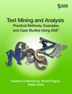
Plotting the documents in the SVD space (Display 6.1) shows that documents D1 and D2 are close together and documents D3 and D4 are close together. Although the task of separating the four documents in the two groups (D1, D2 versus D3, D4) seems easy to do for any English speaker, it is gratifying to see that it can be done reasonably well via SVD.
Display 6.1: Two-Dimensional Plot of Document Coordinates from Table 6.2
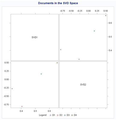
In the plot, SVD1 and SVD2 are shown as the X and Y axes. But, just like in factor analysis, these axes can be rotated to better align the documents with the axes. For example, if you rotate the axes (keeping the angle between them constant at 90 degrees or ensuring zero correlations between SVD1 and SVD2) by about 45 degrees in the plot, the documents align well with the rotated axes as shown in Display 6.2.
Display 6.2: Rotated X and Y Axes for Dimensions in Display 6.1
Recall that these SVDs are the latent semantic dimensions of the text documents. Plotting both documents and terms in the SVD space can provide more insight into how documents and terms are related in the SVD space and the meaning of the latent semantic dimensions. Labels for semantic dimensions are often arrived at subjectively by inspecting plots or by plotting other known and labeled variables in the same SVD space and noting the relationships among these variables and the SVDs. In this example, just by quickly reading the documents aligned closely with each dimension, you can see that one dimension seems to capture the semantic concept of the usefulness of the iPad, and the other dimension seems to capture the semantic concept of playing soccer.
Text Cluster Node
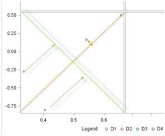
In the process flow, the Text Cluster node must be preceded by the Text Parsing and Text Filter nodes as shown in the process flow diagram in Display 6.3.
Display 6.3: SAS Global Forum Example Process Flow with Text Cluster and Text Topic Nodes
There are two algorithms available for clustering: the hierarchical algorithm and the expectation-maximization (EM) algorithm. The EM algorithm is the default option. In SAS Text Miner, EM clustering automatically selects between two versions of the EM algorithm—standard or scaled. The standard version of the EM algorithm analyzes all data at each iteration step and is used when the data size is small. The scaled version of the EM algorithm uses part of the input data in each iteration and is used when the data is large.
Display 6.4: Text Cluster Node Properties Panel
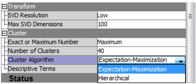
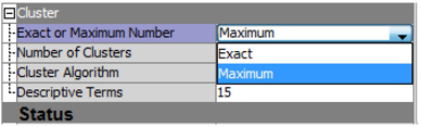
SVD Resolution is set to Low by default, which results in the algorithm automatically selecting to use a minimum number of SVD components (up to a maximum of 100) in the clustering algorithm. One way to think about resolution is how much information you are giving up to reduce the dimensionality of the weighted term-by-document matrix. Low resolution results in more loss of information than high resolution. On the other hand, high resolution means little reduction in dimensionality. As the famous economist Milton Friedman said, “There is no free lunch.” In text analytics problems, you should start with the default setting, and then be prepared to experiment with the maximum number of SVD dimensions and resolution. In the Text Mining node, you can control the number of clusters either by using the Maximum cluster option (the default) with Low SVD resolution or by using the exact number of clusters.
Display 6.5: Cluster Technique Property Settings
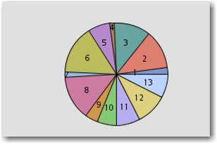
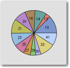
Using the default settings (Low SVD resolution and Maximum cluster) results in 13 clusters with the SAS Global Forum text corpora as shown in Display 6.6.
Display 6.6 Cluster Identified with Default Properties
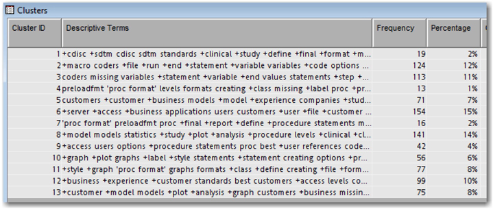
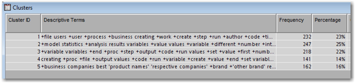
By default, SAS Text Miner uses 15 descriptive terms that best describe each cluster as shown in Display 6.7.
Display 6.7: Descriptive Terms for Clusters Identified with Default Settings
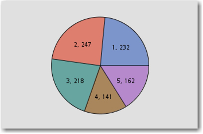
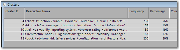
If SVD resolution is set to High, then only five clusters are generated as shown in Display 6.8.
Display 6.8: Five Clusters and Descriptive Terms Identified with High SVD Resolution Setting
The number of clusters generated is usually different, not just based on SVD resolution, but also based on the type of algorithm used. This is expected in unsupervised classification techniques (such as clustering) and underscores the importance of a user’s involvement and judgment that is needed to select the best solution. For the SAS Global Forum corpora, the use of the default setting (low SVD resolution) with hierarchical clustering results in a large number of clusters as shown in Display 6.9.
Display 6.9: Hierarchical Clustering Results with Low SVD Resolution
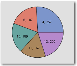
If SVD resolution is set to high, then the number of clusters is reduced to five as shown in Display 6.10. Although the number of clusters in this case happens to be the same as the result of the EM algorithm, note that the frequencies of documents in each cluster and their descriptive terms are quite different.
Display 6.10: Hierarchical Clustering Results with High SVD Resolution
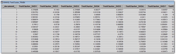
Once you run any clustering on the text corpora, the exported data from the Text Cluster node will contain the SVD values. For example, the SVD values for the SAS Global Forum text corpora for the EM algorithm with low SVD resolution are shown in Display 6.11.
Display 6.11: Text Cluster Node Output Data Set with SVD Values
Many other clustering options (including SOM, k-means, hierarchical methods such as centroid, average, and so on) are available in SAS Enterprise Miner either through stand-alone nodes (such as SOM/Kohonen or k-means) or through the use of a SAS Code node (such as average, centroid, and so on, as the hierarchical clustering option). The exported SVD values from the Text Cluster node can easily be used by analysts to explore other clustering options.
Topic Extraction
In Chapter 5, you learned about and appreciated the benefits of concept links. They help in understanding the relationships between terms based on their co-occurrence in the documents. They are represented in the form of a hub-and-spoke structure, where the strength of the relationship is indicated by the width of the connecting line. The same concept can be extended to understand how various documents are associated to a topic. A topic is a collection of terms that define a theme or an idea. Every document in the corpus can be given a score that represents the strength of association for a topic. A document can contain zero, one, or many topics. The objective of creating a list of topics is to establish combinations of words that are of interest in the analysis. For example, a car manufacturer might want to explore all product reviews to see negative comments on a particular car feature, for example, the navigation system. The analyst can define a topic, “Negative Nav Sys,” using the terms “GPS,” “navigation,” “bad,” “malfunctioning,” “useless,” and “faulty.” You can get a sense of the possible negative terms for defining the topic by browsing the terms table. Display 6.12 illustrates the difference between concept links and text topics by considering the term navigation and the topic “Negative Nav Sys.”
Display 6.12: Similarity between a Concept Link and a Text Topic
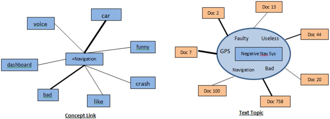
In this example, “Negative Nav Sys” shows a strong association with Document 7, Document 2, and Document 758. The importance of a particular term within a topic is defined by a weight assigned to each term in that topic. A term can be part of multiple topics and therefore gets multiple weights.
Text Topic Node
The Text Topic node in SAS Text Miner discovers topics from text. Fundamentally, the node analyzes document contents and summarizes the collection by identifying topics. The Text Cluster node generates clusters where each document can belong to only one cluster. In a text topic analysis, each document can belong to many topics. The Text Topic node enables an analyst to create topics of interest using groups of terms identified in text parsing. The node can be configured to identify single-term topics or multi-term topics in the data. Topic extraction is a computer-intensive task because the node uses rotated SVD in the background to capture information from a sparse term-by-document matrix. We have discussed in detail the mechanics of SVD in earlier sections of this chapter. Here is the SVD example discussed earlier in this chapter. Suppose you have the following set of four text documents:
D1: I love iPad.
D2: iPad is great for kids.
D3: Kids love to play soccer.
D4: I play soccer at OSU.
With two eigenvalues retained, coordinates of the terms represented in the SVD space are shown.
Table 6.3: Coordinates of Each Term for the Two SVD Dimensions from the Example
| ID | Type | SVD1 | SVD2 |
| I | Term | 0.99 | 0.225 |
| Love | Term | 0.876 | -0.105 |
| iPad | Term | 0.739 | -1.078 |
| is | Term | 1.06 | -0.307 |
| Great | Term | 0.405 | -0.806 |
| Kids | Term | 0.949 | -0.637 |
| Play | Term | 1.197 | 0.667 |
| Soccer | Term | 1.197 | 0.667 |
| OSU | Term | 0.656 | 0.498 |
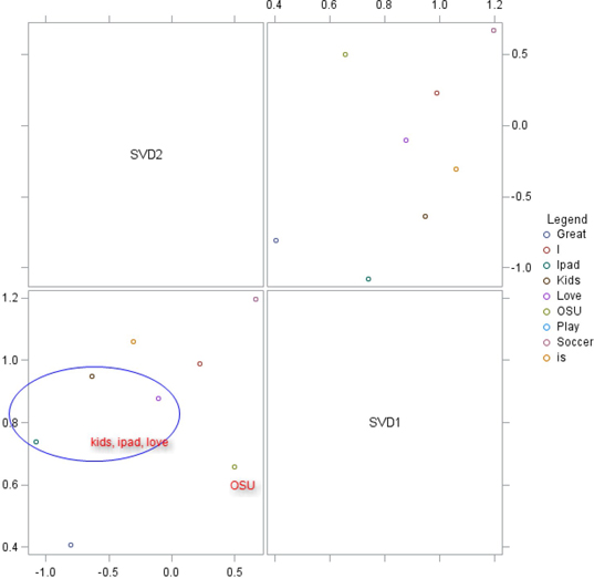
Plotting the terms in the SVD space (as shown in Display 6.13) shows that the terms “iPad,” “kids,” and “love” are close, and the terms occurring only once in the text like “great” and “OSU,” are far from the other terms. The terms “iPad,” “kids,” and “love” can be combined to form a topic. Similarly, the terms “love,” “is,” and “I” can be combined to form another topic.
Display 6.13: Plot of SVD Coordinates from Table 6.3
The Text Topic node must be preceded by either the Text Parsing or Text Filter node. When the Text Topic node is connected to a Text Filter node, the term weighting properties set in the Text Filter node are used by the Text Topic node. Otherwise, default settings (such as Log for frequency weighting and Entropy for term weighting) are used for calculating weights. The properties of the node should be decided carefully based on the size of the document collection.
By default, the node doesn’t generate any single-term topics. You can specify this using the Number of Single-term Topics setting in the Properties panel. You cannot specify more than 1,000 or more than the number of terms imported into the Text Topic node, whichever is smaller. If you want to represent each extracted term in text parsing as a topic, then create that many single-term topics. SVDs are not required for creating single-term topics. They are generated based on the weights calculated for the terms. However, as shown in the previous example, SVDs are essential for creating multi-term topics. The node, by default, creates 25 multi-term topics, where each topic is essentially an SVD dimension. You can always modify this number using the property setting Number of Multi-term Topics.
The requested number should not exceed one of the following:
• 1,000
• the number of documents minus 6
• the number of terms that are imported into the Text Topic node minus 6
Fewer topics are generated than requested in instances where SVD results lead to duplicate topics. To avoid convergence issues, always specify a number that is smaller and not too close to the number of documents and the number of terms that are imported into the Text Topic node.
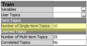
Consider the SAS Global Forum corpus for topics using the Text Topic node. Connect a Text Topic node to the Text Filter node. In the Properties panel (as shown in Display 6.14), set the Number of Single-term Topics property to 10, and run the node. The Correlated Topics property specifies whether topics must be uncorrelated or if they can be correlated.
Display 6.14: The Text Topic Node Train Properties Panel
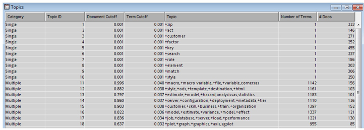
Display 6.15 shows the Topics window from the results window of the Text Topic node. The 10 single-term topics extracted, like “zip,” “act,” “customer,” etc., are at the top of the list, with document cutoff and term cutoff values as 0.001. Multi-term topics like topic 11 talk about macros and macro variables. Topic 14, representing software implementations, contains the terms “server,” “deployment,” “metadata,” and “configuration.” You can see each topic’s multi-term topic containing thousands of terms. Only the top five weighted terms for each topic are shown in the Topic column.
Display 6.15: Topics Table from Text Topic Node Results
To understand the results of the Text Topic node, you need to understand the difference between term topic weight and document topic weight.
Term topic weight: Each term is assigned a weight corresponding to each topic. If there are 25 topics extracted, there will be 25 term topic weights calculated for a single term. Because each topic is an SVD dimension, the term topic weights for a term are nothing but the coordinates of the term in the SVD space. In Table 6.1, the coordinates 0.876 and -0.105 corresponding to the term “love” are the term topic weights corresponding to the two SVD dimensions.
Document topic weight: Similarly, every document in the collection is assigned a weight corresponding to each topic. If there are 25 topics extracted, there will be 25 document topic weights calculated for a single document. The document topic weight of a document toward a topic is the normalized sum of tf-idf weightings for each term in the document multiplied by their term topic weights.
Term topic weights and document topic weights are used to calculate cutoff scores for each multi-term topic.
• Term cutoff: This is the threshold score that determines whether a term belongs to a topic. This is equal to the mean + 1 standard deviation of all term topic weights for that topic. Any term with an absolute term topic weight greater than this cutoff is assigned to this topic.
• Document cutoff: This is the threshold score that determines whether a document belongs to a topic. This is equal to the mean + 1 standard deviation of all document topic weights for that topic. Any document with an absolute document topic weight greater than this cutoff is assigned to this topic.
A better understanding of these weights and cutoffs can be achieved using the interactive topic viewer. An analyst is given complete control to modify these weights to ensure that certain terms are always assigned to or eliminated from a particular topic via the Interactive Topic Viewer.
Interactive Topic Viewer
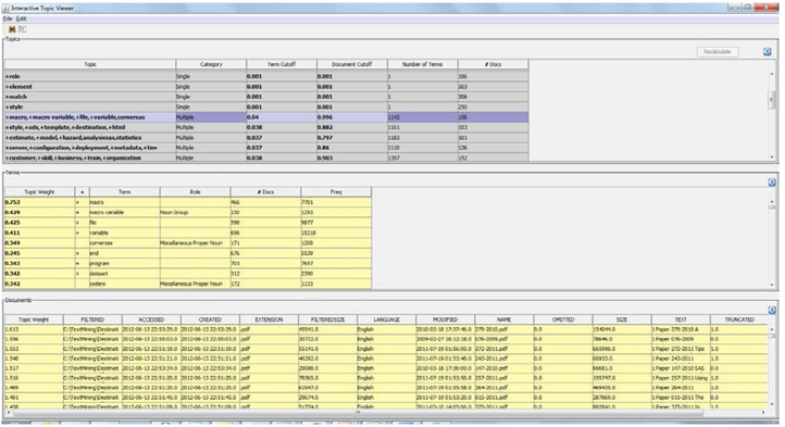
The Text Topic node provides a facility to interactively adjust the topics. Click the ellipsis button next to Topic Viewer in the Properties panel. Display 6.16 shows the Interactive Topic Viewer. This window is divided into three sections: Topics, Terms, and Documents. The contents of the Terms and Documents sections update based on the topic selected in the Topics section. To select a specific topic, right-click on the last column of that particular topic, and select Select current Topic.
Display 6.16: Interactive Topic Viewer
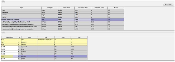
In the Topics section, you can modify the values in only the Topic, Term Cutoff, and Document Cutoff columns. For example, consider the topic “+macro,+macro variable,+file,+variable,cornersas.” You can rename this topic “Macros and Macro variables” by just replacing the text in the Topic field. A Term Cutoff score of 0.04 is calculated for this topic. From the Terms section, all terms with an absolute topic weight value greater than or equal to 0.04 are assigned to this topic. (See Display 6.17.)
Display 6.17: Topic Cutoff for the Topic “+macro,+macro variable,+file,+variable,cornersas”
You can add more terms to this topic by adjusting the cutoff values. For example, to add the term “interface” that has a term topic weight of 0.039, you can change the term cutoff value for this topic in the Topics section to 0.039. By decreasing the term cutoff value, you are effectively increasing the number of eligible terms for the topic. This also impacts the weights of the documents. This change results in all terms with a term topic weight of 0.039 being added to this topic, which is not wanted. However, you can directly adjust the term topic weight value for a specific term in the Terms table. In Display 6.18, the topic weight value for the term “interface” is changed to 0.04.
After the changes, the Category column of the topic Macros and Macro variables shows User in the Topics section because the topic name is modified by the user. Whenever any changes are made to the cutoff values, click Recalculate in the top right corner of the Interactive Topic Viewer for the changes to be applied.
Display 6.18: Interactive Topic Viewer Showing User-Edited Content
Similarly, you can eliminate specific terms from a topic by adjusting the term topic weight to a value outside the term cutoff threshold. Similar operations can be performed for including or excluding documents assigned to a topic that are shown in the Documents section. You can investigate the extracted terms by exploring the actual text from the Documents section.
User-Defined Topics
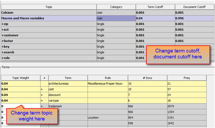
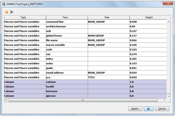
Another great functionality of the Text Topic node is the ability to define custom topics of interest. You can add custom topics directly using the interface or you can import them as a SAS data set. Click the ellipsis button next to the User Topics property from the node’s Properties panel. As shown in Display 6.19, you can see the topic Macros and Macro variables in this table because this topic has been modified by the user. Scroll to the bottom of the window to add a custom topic named Calcium and its associated terms as shown in Display 6.19. Enter a value for the weight for each term. Weight is a relative value between 0 and 1 given to each Role and Term pair that indicates the importance of the term to the topic. A value of 1 indicates high importance, and a value of 0 indicates low importance.
Display 6.19: Creating User-Defined Topics
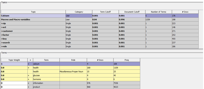
Run the Text Topic node with the user-defined topics. View the Interactive Topic Viewer after the completion of the run. Display 6.20 shows the results from the Interactive Topic Viewer after the node is run with user-defined topics. The user-defined topics are at the top of the Topics table. There are 176 documents that contain the topic Calcium. You can enhance this topic by adding more terms and adjusting the cutoffs.
Display 6.20: Interactive Topic Viewer with User-Defined Topics
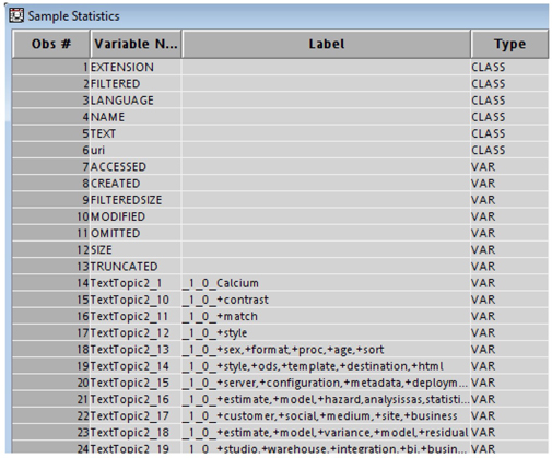
The output data set of the Text Topic node contains new variables that represent topics created by the node. There are two variables created for each topic: one is the document cutoff score and the other is a binary variable indicating topic assignment. The binary variable has a value of 1 if the document topic weight is greater than or equal to the document cutoff score. It has a value of 0 otherwise. In our example, 27 topic binary variables are created. These include two user-defined topics, 10 single-term topics, and 15 multi-term topics. Display 6.21 shows the new topic binary variables in the output data set and the existing text variables. In the presence of a target variable, the topic binary variables lend themselves as valuable input variables for performing structured data mining analysis.
Display 6.21: Topic Binary Variables Created in the Text Topic Node Output Data Set
Scoring
In the last five chapters, you learned how to perform text mining analysis using SAS Text Miner. Like any typical data mining process, the task that follows modeling is scoring. A model is trained using development data, and then it is applied to customer records in a production or live system to calculate a score for each record. An appropriate business action is performed based on the calculated score. Similarly, a text mining process can be scored on new textual data. In the context of text mining, scoring means assigning a document to a cluster or to a topic. The Score node in SAS Enterprise Miner is used for this purpose. A Score node can be connected to either a Text Cluster node or Text Topic node. If the data for scoring resides on a different database system, you can take the score code generated by any of these nodes (Text Cluster or Text Topic or Score node) and run it on the other database system for scoring. These nodes only generate SAS code for scoring. The scoring process is demonstrated using an example in Case Study 9.
Summary
In this chapter, we discussed some of the key technical concepts in text mining analysis used for identifying clusters or topics in the textual corpus. We explained the mechanics of the different clustering algorithms available in SAS Text Miner. We demonstrated the topic extraction functionality in SAS Text Miner. Remember that text mining is an iterative and exploration-oriented analysis. There is no one specific clustering technique or topic extraction setting that yields the best results. Hence, it is always suggested to explore different property settings and techniques. Often, an analyst is required to go back in analysis and modify property selections in the Text Parsing and Text Filter nodes. These changes can alter the term-by-document matrix considerably. Further, these changes have significant impact on the clusters and the topics extracted. Cluster analysis and topic extraction suffer from the curse of dimensionality in the term-by-document matrix. SVD is used to reduce the dimensionality in the term-by-document matrix. Although a higher number of SVDs can summarize the data better, they are not wanted due to computing limitations and the higher risk of fitting the noise. SAS Text Miner provides a user with the ability to control the number of SVDs to use in the analysis.
References
Bradley, P. S., Fayyad, U., & Reina, C. 1998. “Scaling Clustering Algorithms to Large Databases.” KDD 1998: Proceedings of the Fourth ACM SIGKDD International Conference on Knowledge Discovery and Data Mining, 9-15.
Cattell, R. B. 1966. “The Scree Test for the Number of Factors.” Multivariate Behavioral Research. 1(2): 245-276.
Esposito Vinzi, V., Chin, W. W., Henseler, J., & Wang, H. (Eds.) 2010. Handbook of Partial Least Squares: Concepts, Methods, and Applications. New York: Springer. (Springer Handbooks of Computational Statistics).
Everitt, B. S., Landau, S., & Leese, M. 2001. Cluster Analysis. Arnold, London.
Kohonen, T., 1995. “Self-Organizing Maps.” Springer Series in Information Sciences. Vol. 30. Berlin: Springer-Verlag.
Landauer, T. K., Foltz, P. W., & Laham, D. 1998. “An Introduction to Latent Semantic Analysis.” Discourse Processes. 25(2-3): 259-284.
Manning, C. D., & Schütze, H. 1999. Foundations of Statistical Natural Language Processing. Cambridge: MIT Press.
Radovanović, M., & Ivanović, M. 2008. “Text Mining: Approaches and Applications.” Novi Sad Journal of Mathematics. 38(3): 227-234.
Sullivan, D. 2001. Document Warehousing and Text Mining: Techniques for Improving Business Operations, Marketing, and Sales. John Wiley & Sons, Inc.
Text Analytics Using SAS® Text Miner: Course Notes. SAS Institute Inc., Cary, NC. Course information: https://support.sas.com/edu/schedules.html?ctry=us&id=1224