Case Study 1 Text Mining SUGI/SAS Global Forum Paper Abstracts to Reveal Trends
Zubair Shaik
Satish Garla
Goutam Chakraborty
Instructions for Accessing the Case Study Project
Introduction
Text Mining is mainly used for information retrieval and text categorization. With the growth of social media, the popularity of text mining as a technique to discover trends in topics has caught up tremendously. Given a set of documents with a time stamp, text mining can be used to identify trends of different topics that exist in the text and how they change over time. In this case study we aim to demonstrate the application of text mining for understanding trends in conference proceedings.
Many professional conferences or forums are held every year across the globe. The total number of papers presented each year at all the conferences is likely in the hundreds of thousands. While there are conferences which focus on only one specific field, there are many conferences which act as a platform for different fields. Unlike academic journals, which are heavily indexed and searchable, most conference papers are not indexed properly. In addition, there are many academic institutions that publish working papers and many consulting firms that publish white papers every year which are also not indexed. While it may be possible to use a structured query to get a listing of papers published about a certain topic from indexed journals/conferences, it is virtually impossible to gain broad based knowledge about the hundreds of topics that are presented or published during a time period and how such topics may have changed over time.
Data
The data used in this case study are abstracts of all SAS conference papers published each year at SUGI/SAS Global Forum from 1976 to 2011. Initially, we considered three types of textual data for text mining,
• Title of the paper
• Abstract of the paper
• Complete body of the paper
Title of the paper may not be a good input because it is often restricted in length and may not fully reflect the theme of the paper semantically. Considering the complete paper for analysis will likely add a lot of noise because a full paper can include tables, images, references, SAS programs, etc., which are problematic and may not add much value in text mining for topic extraction. We felt analyzing the abstract of a paper to be most appropriate since it captures a detailed objective of the paper and does not contain extraneous items such as tables, images, etc. We are thankful to SAS for making available SUGI/Global Forum proceedings for all of the years the conference was held. We faced many challenges starting from downloading papers in PDF format from the SAS website to preparing a final data set that contains only the abstract for each paper. We used the %TMFILTER macro for preparing SAS data sets from a repository of SAS papers in .pdf and .txt format. We had to make some strategic choices to prepare the data sets. For complete details on the data preparation process refer to 2012 SAS Global Forum paper ‘SAS Since 1976: An application of text mining to reveal trends’. In the paper, the authors created four data sets, one for each decade, with the number of observations (i.e., paper abstracts) shown in Display C1.1.
Display C1.1 Number of paper abstracts in each ecade
For this case study we start with the same four data sets with only one exception, the latest decade data set also includes papers from the 2012 SAS Global Forum conference.
The four data sets used for this analysis are:
• sas1976_1980
• sas1981_1990
• sas1991_2000
• sas2000_2012
The data sets are available in the folder Case Studies ▸ Case Study 1 provided with this book. See the website for this book.
The following sections take you through the detailed, step-by-step text mining process from text parsing to cluster generation on each data set separately.
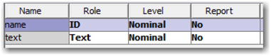
1. Create a SAS Enterprise Miner project and create four data sources using the above data sets. In each data source, set the Role of the variable ‘text’ to Text and the role of the variable ‘name’ to ID, as shown below.
Display C1.2 Variables list window in data source creation
2. Create a Diagram and drag the data source SAS1976_1980 to the diagram workspace.
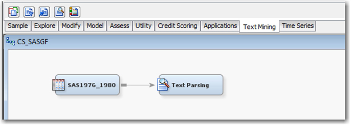
3. Connect a Text Parsing node to the data source node (Display C1.3) and Run the node.
Display C1.3 SAS Enterprise Miner diagram space
4. After the completion of the run, select Results on the Run status dialog box
5. Maximize the Terms window. This window (Display C1.4) contains list of all terms extracted with term properties such as role, attribute, frequency, Keep/Drop status, parent/child status and the rank assigned to the term.
Display C1.4 Terms window
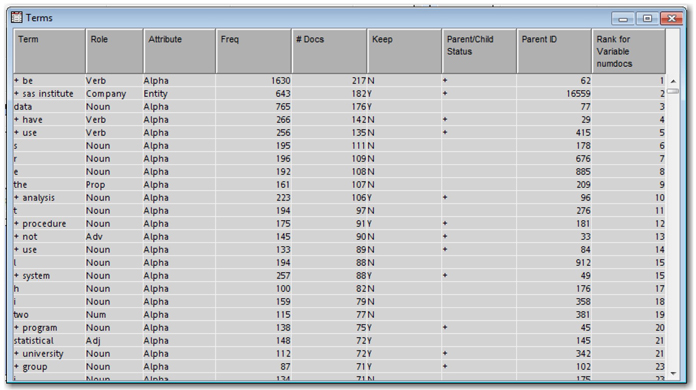
A great deal of understanding about what is happening for the settings being used in the nodes can be made by looking at the Terms table. Once you have a sense of which terms are being kept or dropped and their Role, you can then adjust the settings accordingly. Let us explore how you can make use of the ‘Entity’ extraction property in the parsing node. This property has a default value of ‘None’. In this case study you will not have a need to identify entities since you are analyzing just the abstract of a paper. However, due to limitations in the data preparation task, you will find names of authors, location, company, and address appearing in the text. Most of these entities are parsed as a proper noun when the entity property is disabled. These terms may be considered as noise in our analysis because our interest is in the trend.
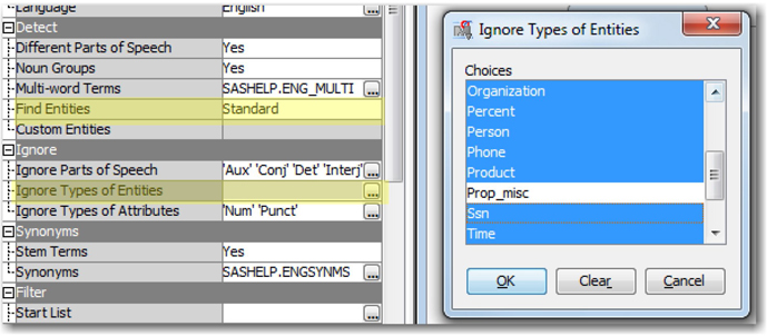
6. Exclude these terms from analysis by changing the ‘Find Entities’ property from None to Standard in the properties panel of the text parsing node. Then, click on the ellipsis button next to ‘Ignore Types of Entities’ and select all terms except Miscellaneous Proper Noun (Prop_misc) as shown in Display C1.5.
Display C1.5 Text Parsing node property panel
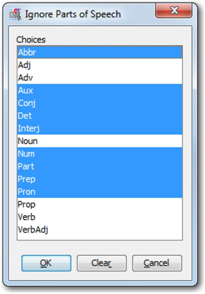
7. Parts of speech will add no value in our current analysis. Hence, set the Different Parts of Speech property to No. With this setting you will find words such as “the”, “an”, “also”, etc, being included in the analysis. You can drop these terms from the analysis by using the ‘Ignore Parts of Speech’ property, as shown in Display C1.6.
Display C1.6 Ignore Parts of Speech property window
When a synonyms list is already available, you can use them with the Text Parsing node. Otherwise these lists can be custom generated for this data using the Text Filter node.
8. Connect a Text Filter node to the Text Parsing node. Enable the spell-checking property and set the Maximum Number of Documents property value 5 and Run the node.
After the run completion, the Interactive Filter Viewer window can be accessed to explore and interactively manage the terms. The main objective is to filter the terms not needed for analysis. Generating a Start/Stop list and a synonym list are integral to this task.
The simplest way to filter words is to select a number of terms from the Terms window and uncheck the Keep column. From the interactive filter window, try sorting the Terms table multiple times for each different column to understand groups of related terms. For example, sorting the ‘Term’ column will help in identifying synonyms that are very close in spelling, such as the terms airline, aviation, aircraft, etc.
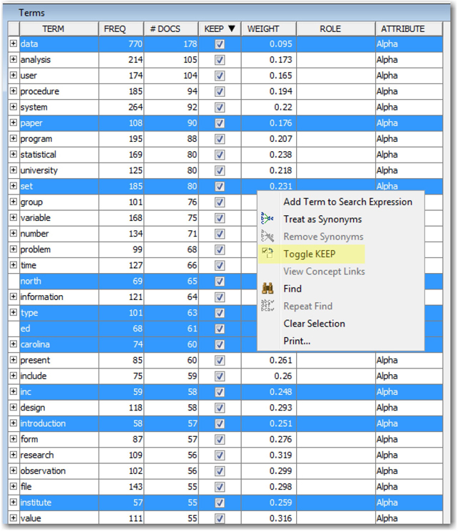
9. Sort the Terms table by the KEEP column. You will see all the terms retained in the analysis in the order of document frequency. Clearly you will always see certain terms that exist across almost all the documents that provide no value in discriminating the documents. In this case, high frequency terms like data, paper can be dropped. Other high frequency terms like set, type, ed, carolina, inc, north, introduction, institute can be dropped since they are not useful in this analysis.
10. Select all these terms as shown in Display C1.7, right-click and select ‘Toggle KEEP’. This will uncheck the KEEP column for all these terms and they are dropped from analysis.
Display C1.7 Terms window from Interactive filter viewer
11. Now sort the Terms table by the TERM column. Scroll down the table to identify similar terms and create a synonym list. Navigate to the terms starting with letter “b” by hitting the letter “B” on the keyboard. Scroll down the list to the term “bio”. You will see a lot of terms with the letters “bio” that can be treated as synonyms. To make all these terms synonyms, select the terms bio, biochemical, biological, biomedical, biometrics, biometrika, biometry, biometries, biostatistics, then right-click and select ‘Treat as Synonyms’ as shown in Display C1.8.
Display C1.8 Terms window showing creating synonyms

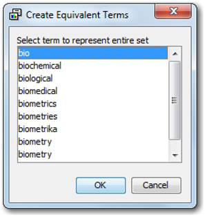
12. In the following dialog (see Display C1.9), select “bio” as the keyword to represent the group. Hence when these terms were represented individually, all the terms were dropped from the analysis due to their low document frequency (less than 5 as in the setting). With the creation of synonym group, the term “bio” will now be considered in the analysis since the document frequency meets the cut-off. You will have to re-run the node to see this term included in your analysis.
Display C1.9 Window to select parent synonym term
Similarly, browse through the complete list of terms to keep the dropped terms and to drop the kept terms wherever appropriate for the analysis. This is the most important and time-consuming task of text mining analysis. This task is purely subjective and completely depends on the problem and the analyst’s level of domain expertise.
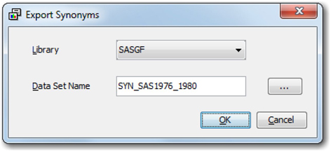
13. In the end, save the custom synonyms by clicking on File ▸ Export Synonyms. Select the Library where you intend to save your work and give a meaningful name to the data set as shown in Display C1.10. Close the interactive filter window and Save all your changes when prompted.
Display C1.10 Creating a custom synonym list
As far as the case study is concerned, it is highly difficult to list all of the operations performed at this stage. Hence we provide you with a custom synonym list that can be used with the Text Filter Node.
14. Connect a Text Cluster node to the Text Filter node. Set the Maximum number of the clusters property to 20 and run the node.
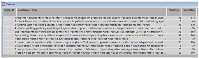
The Results window (see Display C1.11) of the Text Cluster node displays 11 clusters generated by the Expectation – Maximization (EM) method. It is worth trying other methods like Hierarchical clustering with different SVD resolution levels before you conclude on a final result. For EM techniques with Low SVD resolution settings we clearly see a reasonable separation of the documents. As shown in display C1.11 Cluster 8 includes papers on the GLM procedure, linear regression; cluster 2 includes papers on experiments, effects, treatment; cluster 4 contains papers on graphs, plots, line options, etc.
Display C1.11 Cluster results for 1970s data
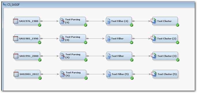
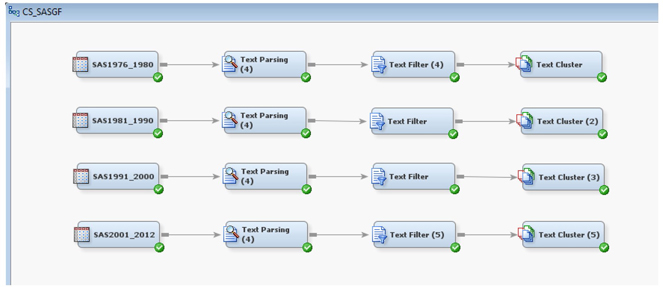
What you have seen up until now is a typical and basic process flow in text mining analysis. By performing these steps, you gain a fair understanding of the text. Since the objective of this case study is to perform trend analysis, carry out the same set of steps with the remaining three data sets, as shown in Display C1.12, representing the latter three decades and compare the results.
Display C1.12 Diagram with process flows for all four decades data
Results
As discussed in Chapter 5, “Data Transformation,” a quick and easy route to understanding the textual data is by looking at the high frequency terms in the corpus. The results window of the Text Parsing node or the Text Filter node can be used to look at the high frequency words. Display C1.13 shows the top occurring terms in each of the four data sets from the Text Filter Node results (only terms that are kept in the analysis are shown here).
Display C1.13 Top frequency terms in each of the four data sets from text filter node
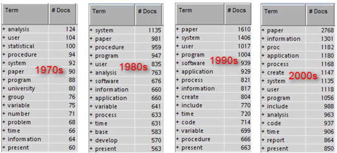
Clearly, there are certain words that occur in all four decades like, system, information, paper, present, program, time, user and procedure. In fact one can exclude all these terms from analysis since these are the common terms that can be easily expected to be present in SAS Conference proceedings. Terms like these definitely do not help in trend detection. However, you will find terms like application, process, and code occurring in all the decades except 1970s. This shows that not a lot of application oriented papers were published in 1970s, rather the papers were more about explaining techniques available in SAS at that time.
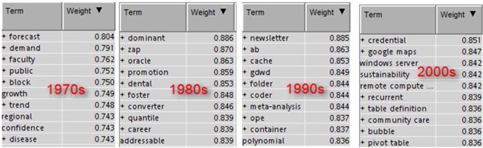
Another way to identify important terms in the text corpus is by looking at the important terms as identified by the term weighting methods. In this case study we used default settings for term weighting methods. It is always recommended to try different settings and explore the results. With default settings, the important terms for four decades are identified as shown below. You can find these in the text filter node results. Just sort the terms file by weight. Clearly, you will see a completely different set of terms identified as important across the four data sets. The weight is calculated using the entropy (default) technique that uses document frequency along with the overall frequency of the terms.
Display C1.14 The most important terms in each of the four data sets from the text filter node
Trends
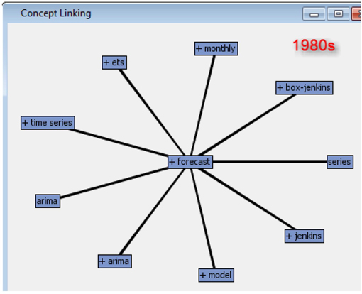
Trends of topics across data sets can be tracked by looking at the frequency of words related to a topic in the four data sets. Another way to explore trends is by understanding the context in which a particular term is frequently used. This can be accomplished by looking at the concept links for a term. You can view the concept links from the interactive filter window (to activate the interactive viewer, in the properties panel for the text filter node, click on the ellipsis button next to Filter Viewer). In the terms window select the term of interest, right-click and select View concept links. Display C1.15 and C1.16 show the concept links for the term “forecast” in the 1980s and 2000s.
Display C1.15 Concept links for the term “forecast” in the 1980s data
Display C1.16 Concept links for the term “forecast” in the 2000s data
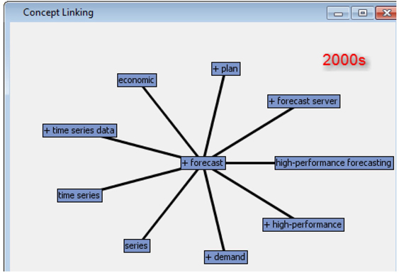
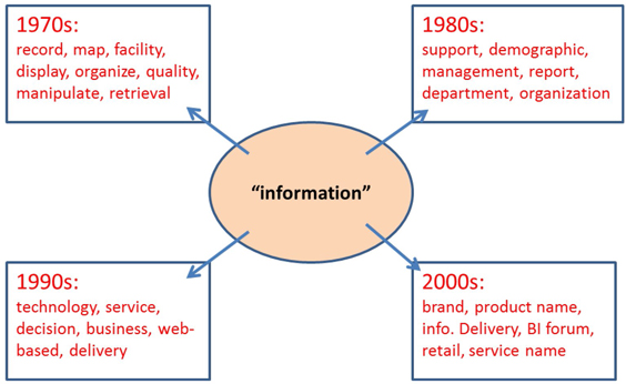
In the 1980s the papers that talked about “forecasting” discussed the technique that is clear from the associated terms like arima, Box-Jenkins, time series, etc., whereas in the 2000s the papers on “forecasting” talked about demand, economic, high-performance forecasting, etc. Similarly, if you observe the term “information”, as shown in Display C1.17, you will understand the context in which the term is heavily used in the conference papers across the four decades.
Display C1.17 Associated terms for the term “information” from all four data sets
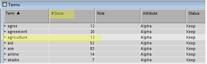
Trends in industry can be explored by creating synonyms using terms related to a specific industry or simply counting the frequencies of various terms that represent a particular industry. The occurrences of industry-specific terms across the four decades can be used to understand the trend for that industry. A frequency value of “n” for a term means that particular term was mentioned in the abstracts of “n” distinct conference papers. The frequency value here is not the overall occurrence of the term, but the number of documents that the term occurs. This value can be obtained from #Docs column from the Terms window of the Text Parsing or the Text Filter node results.
For example, open the results window of the Text Filter node from the 2000s process flow. In the Terms window sort the table by Term column in A to Z order by clicking on the column header. Scroll down to the term “agriculture.” As shown in Display C1.18, the term “agriculture” appears in 12 documents (#Docs).You can easily copy and paste the whole Terms table to a spreadsheet and calculate the percentage of occurrence for each term. In 2000s there are a total of 3,887 terms and, therefore, the percent of occurrence of the term “agriculture” is about 0.31 as shown in Display C1.19.
Display C1.18 Terms window
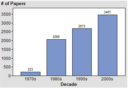
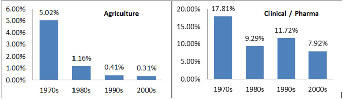
Display C1.19 shows the representation count for the terms “agriculture” and “clinical/pharmaceutical” across the decades. The values in the chart represent the percentage of the papers with these topics compared to the total conference proceedings for the decade. It is clearly evident that the number of papers on agriculture decreased greatly with the years.
Display C1.19 Representation trend for the topic “Agriculture” and “Clinical/Pharmaceutical”
Similarly, you can identify the trend for other industries such as manufacturing, education, health, entertainment, etc. Insights on the trends at a very high level can be gained by looking at the clusters generated for each data set. The theme of each cluster can be understood from the descriptive terms reported by SAS Text Miner. You can request SAS Text Miner to report as many terms as needed in order to describe a cluster. In this analysis we used eight terms to describe a cluster. Earlier in Display C1.17 you saw the cluster results for the 1970s. Display C1.20 shows the clusters generated for the 1980s.
Display C1.20 Cluster results for 1980s data
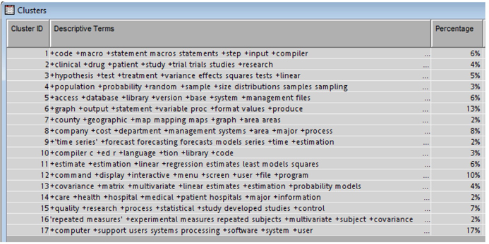
In contrast to statistical techniques and experimentation papers that you have seen in clusters from 1970s, you now see more papers on computer processing (cluster 17), time series forecasting (cluster 9), C-programming (cluster 10), database management (cluster 5) etc., Though you can make a high-level guess on the kind of representation using clusters, a deep understanding on the trend can only be achieved by looking at the terms via concept links and frequencies. The clusters from the latter decades highlight papers on the internet, web-application development, retail, manufacturing, social media etc.
Summary
In this case study you applied text mining to figure out trends in research topics related to various industries in SAS/SUGI conference papers. This case study is intended to showcase the capabilities in SAS Text Miner to track trends of topics in text corpus from different periods of time. The concept links feature of SAS Text Miner is a great tool to discover the context in which a particular term/topic is frequently used. Generating a synonym list on the go makes the text mining analysis more objective. This analysis can be easily extended to find trends in research topics related to different methods or technology. A similar approach can also be used to analyze the many conference proceedings corpus that is available with various organizations across the globe.
Instructions for Accessing the Case Study Project
Along with this book we provide you with both the data used and the SAS Enterprise Miner project created for this case study. The case study includes most of the steps performed in this analysis. However, it is highly impossible to include every single operation performed in text filtering stage. Hence if you start with the data and follow the steps in the case study your results may not match the ones in the case study. Nevertheless, you can use the project to view the exact results presented in the case study. The following instructions will guide you on how to access the project.
1. In the data provided with this book go to the folder Case Studies ▸ Case Study 1. You will find all the data sources needed for this case study and a folder SASGF_Case. The folder is the SAS Enterprise Miner project.
2. Open SAS® Enterprise Miner and click New Project.
3. As shown below enter project name as SASGF_Case and enter the path to the folder and Click Next
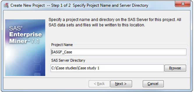
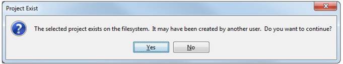
4. You will see the below prompt window. Click Yes.
If you do not see this prompt, then you may have used a different name/path and then this project may not work correctly.
5. Click Next on the following windows and finally click Finish.
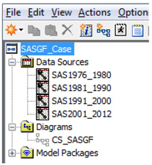
6. The project panel should contain four data sets and one diagram as shown below.
7. Before you run the process flow, you will have to create a library that points to these data sets.
8. Go to Project Start code from the property panel.
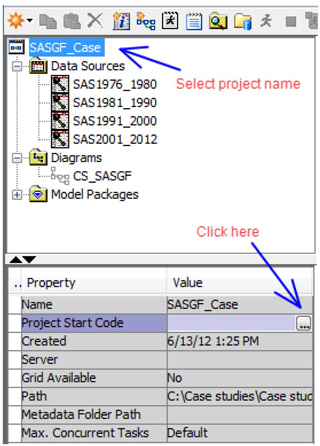
9. Modify the LIBNAME statement with the path pointing to the data folder as shown below and click Run Now.
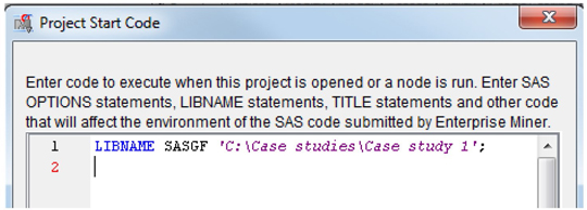
NOTE: If you are using a different LIBREF instead of “SASGF”, you will have to delete the existing data sources and create each data source again using the new LIBREF. You will also have to update the Exported Synonyms property of the Text Filter node to point to the respective decade’s synonyms data set. Hence we suggest using SASGF as the library name for this case study.
10. From the Log tab on Project Start Code window verify that the library was created successfully. Then click Ok.
11. Open the Diagram and run the Text Cluster node for each process as shown below.
You can now view the results for each node as reported in the case study.