Perhaps one of the most widely studied option pricing models is the Black-Scholes-Merton model, or simply the Black-Scholes model in short. A call (put) option is a right, not an obligation, to buy (sell) the underlying security at a particular price and at a particular time. The Black-Scholes model helps determine the fair price of an option with the assumption that returns of the underlying security are normally distributed (N(.)) or that asset prices are log-normally distributed.

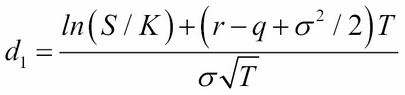
The formula takes on the following assumed variables: the strike price (K), time to expiry (T), risk-free rate (r), volatility of the underlying returns (), current price of the underlying asset (S), and its yield (q). The mathematical formula for a call option is represented as follows:

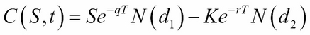
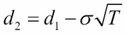
Here:

By way of market forces, the price of an option may deviate from the price derived from the Black-Scholes formula. In particular, the realized volatility (that is, the observed volatility of the underlying returns from historical market prices) could differ from the volatility value as implied by the Black-Scholes model, which is indicated by .

Remember the CAPM model discussed in Chapter 2, The Importance of Linearity in Finance. In general, securities that have higher returns exhibit higher risk, as indicated by the volatility or standard deviation of returns.

With volatility being such an important factor in security pricing, many volatility models have been proposed for studies. One such model is the implied volatility modeling of option prices.

Suppose we plot the implied volatility values of an equity option given by the Black-Scholes formula with a particular maturity for every strike price available. In general, we get a curve commonly known as the volatility smile due to its shape:

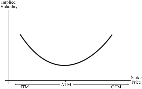
The implied volatility typically is its highest for deep in-the-money (ITM) and out-of-the-money (OTM) options driven by heavy speculation and at its lowest for at-the-money (ATM) options.

From the preceding volatility curve, one of the objectives in implied volatility modeling is to seek the lowest implied volatility value possible or, in other words, to "find the root". When found, the theoretical price of an ATM option for a particular maturity can be deduced and compared against the market prices for potential opportunities, such as for studying near ATM options or far OTM options. However, since the curve is nonlinear, linear algebra cannot adequately solve for the root. We will take a look at a number of root-finding methods in the later sections of this chapter.

To model nonlinear behavior in economic and financial time series, Markov switching models can be used to characterize time series in different states of the world or regimes. Examples of such states could be a volatile state as seen in the 2008 global economic downturn, or a growth state of a steadily recovering economy. The ability to transit between these structures lets the model capture complex dynamic patterns.

The Markov property of stock prices implies that only the present values are relevant for predicting the future. Past stock price movements are irrelevant to the way the present has emerged.

Let's take an example of a Markov regime-switching model with regimes:

is an independent and identically distributed (i.i.d) white noise. White noise is a normally distributed random process with a mean of zero. The same model can be represented with dummy variables:

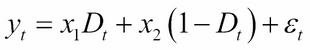
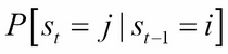
The application of Markov switching models includes representing the real GDP growth rate and inflation rate dynamics. These models in turn drive the valuation models of interest-rate derivatives. The probability of switching from the previous state to the current state can be written as follows:

One popular class of nonlinear time series models is the threshold autoregressive (TAR) model, which looks very similar to the Markov switching models. Using regression methods, simple AR models are arguably the most popular models to explain nonlinear behavior. Regimes in the threshold model are determined by past values of its own time series, relative to a threshold value . The following is an example of a self-exciting TAR (SETAR) model. The SETAR model is self-exciting because switching between different regimes depends on the past values of its own time series:

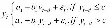
Using dummy variables, the SETAR model can also be represented as follows:

Note that the use of the TAR model may result in sharp transitions between the states as controlled by the threshold variable .

Abrupt regime changes in the threshold models appear to be unrealistic against real-world dynamics. This problem can be overcome by introducing a smoothly changing continuous function from one regime to another. The SETAR model becomes a logistic smooth transition threshold autoregressive (LSTAR) model with the logistic function :

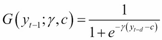
The SETAR model now becomes a LSTAR model, as shown in the following equation:

The parameter controls the smooth transition from one regime to another. For large values of , the transition is the fastest, as approaches the threshold variable . When , the LSTAR model is equivalent to a simple AR(1) one-regime model.