
Nonlinear dynamics plays a vital role in our world. Linear models are often employed in economics due to their simplicity for studies and easier modeling capabilities. In finance, linear models are widely used to help price securities and perform optimal portfolio allocation, among other useful things. One of the significance of linearity in financial modeling is its assurance that a problem terminates at a global optimal solution.
In order to perform prediction and forecasting, regression analysis is widely used in the field of statistics to estimate relationships among variables. With an extensive mathematics library being one of Python's greatest strength, Python is frequently used as a scientific scripting language to aid in these problems. Modules such as the SciPy and NumPy packages contain a variety of linear regression functions for data scientists to work with.
In traditional portfolio management, the allocation of assets follows a linear pattern, and investors have individual styles of investing. We can state the problem of portfolio allocation into a system of linear equations, containing either equalities or inequalities. These linear systems can then be represented in a matrix form as ![]() , where
, where ![]() is our known coefficient value,
is our known coefficient value, ![]() is the observed result, and
is the observed result, and ![]() is the vector of values that we want to find out. More often than not,
is the vector of values that we want to find out. More often than not, ![]() contains the optimal security weights to maximize our utility. Using matrix algebra, we can efficiently solve for
contains the optimal security weights to maximize our utility. Using matrix algebra, we can efficiently solve for ![]() using either direct or indirect methods.
using either direct or indirect methods.
In this chapter, we will cover the following topics:
- Examining the CAPM model with the efficient frontier and capital market line
- Solving for the security market line using regression
- Examining the APT model and performing a multivariate linear regression
- Understanding linear optimization in portfolio allocation
- Linear optimization using the PuLP package
- Understanding the outcomes of linear programming
- Introduction to integer programming
- Implementing a linear integer programming model with binary conditions
- Solving systems of linear equations with equalities using matrix linear algebra
- Solving systems of linear equations directly with the LU, Cholesky, and QR decomposition
- Solving systems of linear equations indirectly with the Jacobi and Gauss-Seidel method
Many financial literatures devote exclusive discussions to the capital asset pricing model (CAPM). In this section, we will explore the key concepts that highlight the importance of linearity in finance.
In the famous CAPM, the relationship between risk and rates of returns in a security is described as follows:
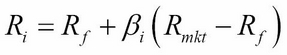
For a security ![]() , its returns is defined as
, its returns is defined as ![]() and its beta as
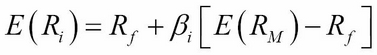
and its beta as ![]() . The CAPM defines the return of the security as the sum of the risk-free rate
. The CAPM defines the return of the security as the sum of the risk-free rate ![]() and the multiplication of its beta with the risk premium. The risk premium can be thought of as the market portfolio's excess returns exclusive of the risk-free rate. The following figure is a visual representation of the CAPM:
and the multiplication of its beta with the risk premium. The risk premium can be thought of as the market portfolio's excess returns exclusive of the risk-free rate. The following figure is a visual representation of the CAPM:
Beta is a measure of the systematic risk of a stock; a risk that cannot be diversified away. In essence, it describes the sensitivity of stock returns with respect to movements in the market. For example, a stock with a beta of zero produces no excess returns regardless of the direction the market moves—it can only grow at the risk-free rate. A stock with a beta of 1 indicates that the stock moves perfectly with the market.
The beta is mathematically derived by dividing the covariance of returns between the stock and the market with the variance of the market returns.
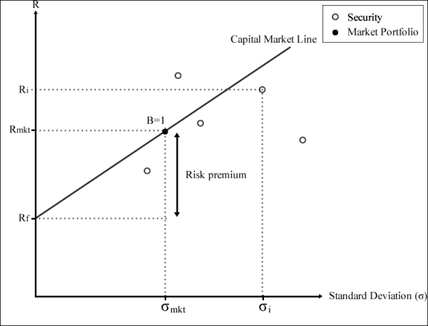
The CAPM model measures the relationship between risk and stock returns for every stock in the portfolio basket. By outlining the sum of this relationship, we obtain combinations or weights of risky securities that produce the lowest portfolio risk for every level of portfolio return. An investor who wishes to receive a particular return would own one such combination of an optimal portfolio that provides the least risk possible. The combinations of optimal portfolios lie along a line called the efficient frontier.
Along the efficient frontier, there exists a tangent point that denotes the best optimal portfolio available giving the highest rate of return in exchange for the lowest risk possible. This optimal portfolio at the tangent point is known as the market portfolio.
There exists a straight line drawn from the market portfolio to the risk-free rate. This line is called the capital market line (CML). The CML can be thought of as the highest Sharpe ratio available among all the other Sharpe ratios of optimal portfolios. The Sharpe ratio is a risk-adjusted performance measure defined as the portfolio's excess returns over the risk-free rate per unit of its risk in standard deviations. Investors are particularly interested in holding the combinations of assets along the CML line. Let's take a look at the following graphical figure:
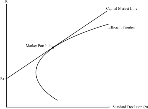
Another line of interest in CAPM studies is the security market line (SML). The SML plots the asset's expected returns against its beta. For a security with a beta value of 1, its returns perfectly match the market's returns. Any security priced above the SML is deemed to be undervalued since investors expect a higher return given the same amount of risk. Conversely, any security priced below the SML is deemed to be overvalued:
Suppose we are interested in finding the beta ![]() of a security. We can regress the company's stock returns
of a security. We can regress the company's stock returns ![]() against the market's returns
against the market's returns ![]() along with an intercept
along with an intercept ![]() in the form the equation
in the form the equation ![]() .
.
Consider the set of stock return and market return data measured over five time periods:
|
Time period |
Stock returns |
Market returns |
|---|---|---|
|
1 |
0.065 |
0.055 |
|
2 |
0.0265 |
-0.09 |
|
3 |
-0.0593 |
-0.041 |
|
4 |
-0.001 |
0.045 |
|
5 |
0.0346 |
0.022 |
Using the stats module of SciPy, we will perform a least squares regression on the CAPM model, and derive the values of ![]() and
and ![]() by running the following code in Python:
by running the following code in Python:
""" Linear regression with SciPy """
from scipy import stats

stock_returns = [0.065, 0.0265, -0.0593, -0.001, 0.0346]
mkt_returns = [0.055, -0.09, -0.041, 0.045, 0.022]

beta, alpha, r_value, p_value, std_err =
    stats.linregress(stock_returns, mkt_returns)
The scipy.stats.linregress function returns the slope of the regression line, the intercept of the regression line, the correlation coefficient, the p-value for a hypothesis test with null hypothesis of a zero slope, and the standard error of the estimate. We are interested in finding the slope and intercept of the line:
>>> print beta, alpha
0.507743187877  -0.00848190035246
The beta of the stock is 0.5077.
The equation describing the SML can be written as:
The term ![]() is the market risk premium, and
is the market risk premium, and ![]() is the expected return on the market portfolio.
is the expected return on the market portfolio. ![]() is the return on the risk-free rate,
is the return on the risk-free rate, ![]() is the expected return on asset
is the expected return on asset ![]() , and
, and ![]() is the beta of asset.
is the beta of asset.
Suppose the risk-free rate is 5 percent and the market risk premium is 8.5 percent. What is the expected return of the stock? Based on the CAPM, the equity with a beta of 0.5077 would have a risk premium of ![]() , or 4.3 percent. The risk-free rate is 5 percent, so the expected return on the equity is 9.3 percent.
, or 4.3 percent. The risk-free rate is 5 percent, so the expected return on the equity is 9.3 percent.
Should the security be observed in the same time period to have a higher return (for example, 10.5 percent) than the expected stock return, the security can be said to be undervalued, since the investor can expect greater return for the same amount of risk.
Conversely, should the return of the security be observed to have a lower return (for example, 7 percent) than the expected return as implied by the SML, the security can be said to be overvalued. The investor receives less return for assuming the same amount of risk.