
Finite difference schemes are very much similar to trinomial tree options pricing, where each node is dependent on three other nodes with an up movement, a down movement, and a flat movement. The motivation behind the finite differencing is the application of the
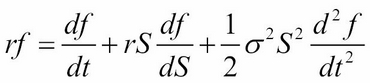
Black-Scholes Partial Differential Equation (PDE) framework (involving functions and their partial derivatives) whose price ![]() is a function of
is a function of ![]() , with
, with ![]() as the risk-free rate,
as the risk-free rate, ![]() as the time to maturity, and
as the time to maturity, and ![]() as the volatility of the underlying security:
as the volatility of the underlying security:
The finite difference technique tends to converge faster than lattices and approximates complex exotic options very well.
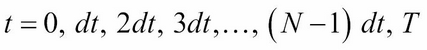
To solve a PDE by finite differences working backward in time, a discrete-time grid of size ![]() by
by ![]() is set up to reflect asset prices over a course of time, such that
is set up to reflect asset prices over a course of time, such that ![]() and
and ![]() take on the following values at each point on the grid:
take on the following values at each point on the grid:
It follows that by grid notation, ![]() .
. ![]() is a suitably large asset price that cannot be reached by the maturity time,
is a suitably large asset price that cannot be reached by the maturity time, ![]() .
. ![]() and
and ![]() are thus intervals between each node in the grid, incremented by price and time respectively. The terminal condition at expiration time
are thus intervals between each node in the grid, incremented by price and time respectively. The terminal condition at expiration time ![]() for every value of
for every value of ![]() is
is ![]() for a call option with strike
for a call option with strike ![]() and
and ![]() for a put option. The grid traverses backward from the terminal conditions, complying with the PDE while adhering to the boundary conditions of the grid, such as the payoff from an early exercise.
for a put option. The grid traverses backward from the terminal conditions, complying with the PDE while adhering to the boundary conditions of the grid, such as the payoff from an early exercise.
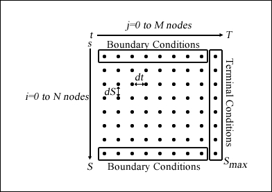
The boundary conditions are defined values at the extreme ends of the nodes, where i=0 and i=N for every time at t. Values at the boundaries are used to calculate the values of all other lattice nodes iteratively using the PDE.
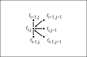
A visual representation of the grid is given by the following figure. As i and j increase from the top-left corner of the grid, the price S tends toward Smax (the maximum price possible) at the bottom-right corner of the grid:
A number of ways to approximate the PDE are as follows:
- Forward difference:
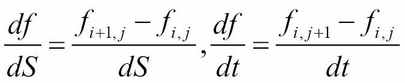
- Backward difference:
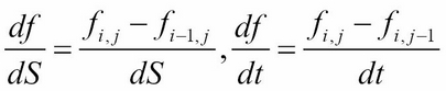
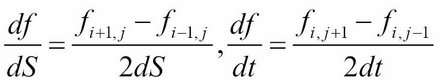
- Central or symmetric difference:
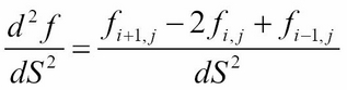
- The second derivative:
Once we have the boundary conditions set up, we can now apply an iterative approach using the explicit, implicit, or Crank-Nicolson method.
The explicit method for approximating ![]() is given by:
is given by:
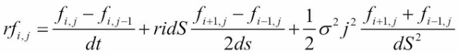
Here, it can be seen that the first difference is the backward difference with respect to ![]() , the second difference is the central difference with respect to
, the second difference is the central difference with respect to ![]() , and the third difference is the second-order difference with respect to
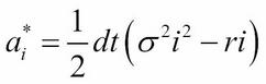
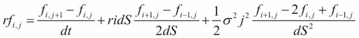
, and the third difference is the second-order difference with respect to ![]() . When we rearrange the terms, we have the following equation:
. When we rearrange the terms, we have the following equation:
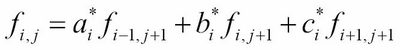
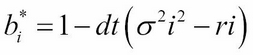
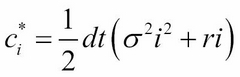
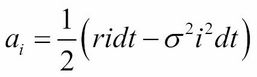
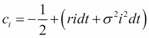
where ![]() and
and ![]() :
:
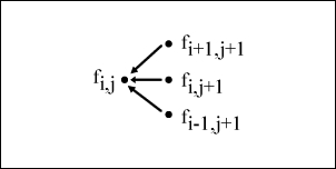
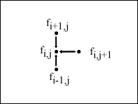
The iterative approach of the explicit method can be visually represented by the following figure:
As we will be writing the explicit, implicit, and Crank-Nicolson methods of finite differences in Python, let's write a parent class that can inherit the common properties and functions of all three methods.
We will create a class called FiniteDifferences that accepts and assigns all the required parameters in the __init__ constructor method and save it as FiniteDifferences.py.
The price method is the public method used for calling the specific finite difference scheme implementation. It will invoke these methods in the following order: _setup_boundary_conditions, _setup_coefficients_, _traverse_grid_, and _interpolate_. These methods are explained as follows:
_setup_boundary_conditions_: This method sets up the boundary conditions of the grid structure as a NumPy two-dimensional array_setup_coefficients_: This method sets up the necessary coefficients used for traversing the grid structure_traverse_grid_: This method iterates the grid structure backward in time, storing the calculated values toward the first column of the grid_interpolate_: Using the final calculated values on the first column of the grid, this method will interpolate these values to find the option price that closely infers the initial stock price, S0
All of these methods are protected methods and may be overwritten by derived classes. The pass keyword simply does nothing; the derived classes will provide specific implementations of these functions:
""" Shared attributes and functions of FD """
import numpy as np


class FiniteDifferences(object):

    def __init__(self, S0, K, r, T, sigma, Smax, M, N,
                 is_call=True):
        self.S0 = S0
        self.K = K
        self.r = r
        self.T = T
        self.sigma = sigma
        self.Smax = Smax
        self.M, self.N = int(M), int(N)  # Ensure M&N are integers
        self.is_call = is_call

        self.dS = Smax / float(self.M)
        self.dt = T / float(self.N)
        self.i_values = np.arange(self.M)
        self.j_values = np.arange(self.N)
        self.grid = np.zeros(shape=(self.M+1, self.N+1))
        self.boundary_conds = np.linspace(0, Smax, self.M+1)

    def _setup_boundary_conditions_(self):
        pass

    def _setup_coefficients_(self):
        pass

    def _traverse_grid_(self):
        """  Iterate the grid backwards in time """
        pass

    def _interpolate_(self):
        """
        Use piecewise linear interpolation on the initial
        grid column to get the closest price at S0.
        """
        return np.interp(self.S0,
                         self.boundary_conds,
                         self.grid[:, 0])
    def price(self):
        self._setup_boundary_conditions_()
        self._setup_coefficients_()
        self._traverse_grid_()
return self._interpolate_()The Python implementation of finite differences by the explicit method is given in the following FDExplicitEu class, which inherits from the FiniteDifferences class and overrides the required implementation methods. Save this file as FDExplicitEu.py:
""" Explicit method of Finite Differences """
import numpy as np

from FiniteDifferences import FiniteDifferences


class FDExplicitEu(FiniteDifferences):

    def _setup_boundary_conditions_(self):
        if self.is_call:
            self.grid[:, -1] = np.maximum(
                self.boundary_conds - self.K, 0)
            self.grid[-1, :-1] = (self.Smax - self.K) *
                                 np.exp(-self.r *
                                        self.dt *
                                        (self.N-self.j_values))
        else:
            self.grid[:, -1] =
                np.maximum(self.K-self.boundary_conds, 0)
            self.grid[0, :-1] = (self.K - self.Smax) *
                               np.exp(-self.r *
                                      self.dt *
                                      (self.N-self.j_values))

    def _setup_coefficients_(self):
        self.a = 0.5*self.dt*((self.sigma**2) *
                              (self.i_values**2) -
                              self.r*self.i_values)
        self.b = 1 - self.dt*((self.sigma**2) *
                              (self.i_values**2) +
                              self.r)
        self.c = 0.5*self.dt*((self.sigma**2) *
                              (self.i_values**2) +
                              self.r*self.i_values)

    def _traverse_grid_(self):
        for j in reversed(self.j_values):
            for i in range(self.M)[2:]:
                self.grid[i,j] = self.a[i]*self.grid[i-1,j+1] +
                                 self.b[i]*self.grid[i,j+1] +
                                 self.c[i]*self.grid[i+1,j+1]
On completion of traversing the grid structure, the first column contains the present value of the initial asset prices at t=0. The interp function of NumPy is used to perform a linear interpolation to approximate the option value.
Besides using linear interpolation as the most common choice for the interpolation method, the other methods such as the spline or cubic may be used to approximate the option value.
Consider the example of an European put option. The underlying stock price is $50 with a volatility of 40 percent. The strike price of the put option is $50 with an expiration time of 5 months. The risk-free rate is 10 percent.
We can price the option using the explicit method with a Smax value of 100, an M value of 1000, and a N value of 100:
>>> from FDExplicitEu import FDExplicitEu
>>> option = FDExplicitEu(50, 50, 0.1, 5./12., 0.4, 100, 100,
...                       1000, False)
>>> print option.price()
4.07288227815
What happens when other values of M and N are chosen improperly?
>>> option = FDExplicitEu(50, 50, 0.1, 5./12., 0.4, 100, 100,
...                       100, False)
>>> print option.price()
-1.62910770723e+53
It appears that the explicit method of the finite difference scheme suffers from instability problems.
The instability problem of the explicit method can be overcome using the forward difference with respect to time. The implicit method for approximating ![]() is given by:
is given by:
Here, it can be seen that the only difference between the implicit and explicit approximating scheme lies in the first difference, where the forward difference with respect to ![]() is used in the implicit scheme. When we rearrange the terms, we have the following expression:
is used in the implicit scheme. When we rearrange the terms, we have the following expression:
Here, ![]() and
and ![]()
The iterative approach of the implicit scheme can be visually represented by the following figure:
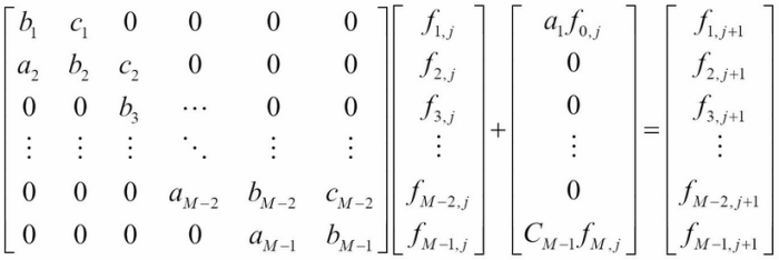
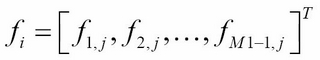
From the figure, it is intuitive to note that values of ![]() are required to be computed before they can be used in the next iterative step, as the grid traverses backward. In the implicit scheme, the grid can be thought of as representing a system of linear equations at each iteration, as follows:
are required to be computed before they can be used in the next iterative step, as the grid traverses backward. In the implicit scheme, the grid can be thought of as representing a system of linear equations at each iteration, as follows:
By rearranging the terms, we get the following equation:
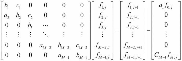
The linear system of equations can be represented in the form of ![]() , where we want to solve for values of
, where we want to solve for values of ![]() in each iteration. Since the matrix A is tri-diagonal, we can use the LU factorization, where A=LU, for faster computation. Remember that we solved the linear system of equations using the LU decomposition in Chapter 2, The Importance of Linearity in Finance.
in each iteration. Since the matrix A is tri-diagonal, we can use the LU factorization, where A=LU, for faster computation. Remember that we solved the linear system of equations using the LU decomposition in Chapter 2, The Importance of Linearity in Finance.
The Python implementation of the implicit scheme is given in the following FDImplicitEu class. We can inherit the implementation of the explicit method from the FDExplicitEu class discussed earlier and override the necessary methods of interest, namely the _setup_coefficients_ and _traverse_grid_ methods:
"""
Price a European option by the implicit method
of finite differences.
"""
import numpy as np
import scipy.linalg as linalg
from FDExplicitEu import FDExplicitEu
class FDImplicitEu(FDExplicitEu):
def _setup_coefficients_(self):
self.a = 0.5*(self.r*self.dt*self.i_values -
(self.sigma**2)*self.dt*(self.i_values**2))
self.b = 1 +
(self.sigma**2)*self.dt*(self.i_values**2) +
self.r*self.dt
self.c = -0.5*(self.r * self.dt*self.i_values +
(self.sigma**2)*self.dt*(self.i_values**2))
self.coeffs = np.diag(self.a[2:self.M], -1) +
np.diag(self.b[1:self.M]) +
np.diag(self.c[1:self.M-1], 1)
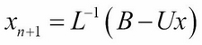
def _traverse_grid_(self):
""" Solve using linear systems of equations """
P, L, U = linalg.lu(self.coeffs)
aux = np.zeros(self.M-1)
for j in reversed(range(self.N)):
aux[0] = np.dot(-self.a[1], self.grid[0, j])
x1 = linalg.solve(L, self.grid[1:self.M, j+1]+aux)
x2 = linalg.solve(U, x1)
self.grid[1:self.M, j] = x2Using the same example as with the explicit scheme, we can price an European put option using the implicit scheme:
>>> from FDImplicitEu import FDImplicitEu
>>> option = FDImplicitEu(50, 50, 0.1, 5./12., 0.4, 100, 100,
...                       100, False)
>>> print option.price()
4.06580193943
>>> option = FDImplicitEu(50, 50, 0.1, 5./12., 0.4, 100, 100,
...                       1000, False)
>>> print option.price()
4.07159418805
Given the current parameters and input data, it is observed that there are no stability issues with the implicit scheme.
Another way of avoiding the instability issue, as seen in the explicit method, is to use the Crank-Nicolson method. The Crank-Nicolson method converges much more quickly using a combination of the explicit and implicit methods, taking the average of both. This leads us to the following equation:
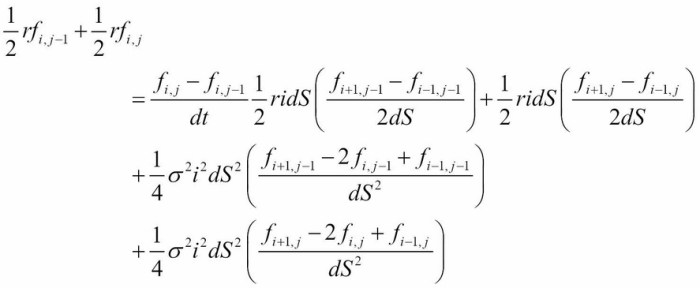
This equation can also be rewritten as follows:
Here:

The iterative approach of the implicit scheme can be visually represented by the following figure:
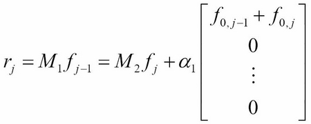
We can treat the equations as a system of linear equations in a matrix form:
Here:
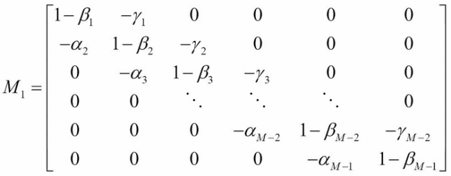
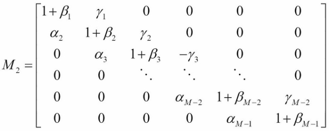
We can solve for the matrix M on every iterative procedure.
The Python implementation of the Crank-Nicolson method is given in the following FDCnEu class, which inherits from the FDExplicitEu class and overrides only the _setup_coefficients_ and _traverse_grid_ methods. Save this file as FDCnEu.py:
""" Crank-Nicolson method of Finite Differences """
import numpy as np
import scipy.linalg as linalg
from FDExplicitEu import FDExplicitEu
class FDCnEu(FDExplicitEu):
def _setup_coefficients_(self):
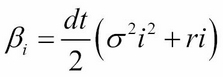
self.alpha = 0.25*self.dt*(
(self.sigma**2)*(self.i_values**2) -
self.r*self.i_values)
self.beta = -self.dt*0.5*(
(self.sigma**2)*(self.i_values**2) +
self.r)
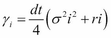
self.gamma = 0.25*self.dt*(
(self.sigma**2)*(self.i_values**2) +
self.r*self.i_values)
self.M1 = -np.diag(self.alpha[2:self.M], -1) +
np.diag(1-self.beta[1:self.M]) -
np.diag(self.gamma[1:self.M-1], 1)
self.M2 = np.diag(self.alpha[2:self.M], -1) +
np.diag(1+self.beta[1:self.M]) +
np.diag(self.gamma[1:self.M-1], 1)
def _traverse_grid_(self):
""" Solve using linear systems of equations """
P, L, U = linalg.lu(self.M1)
for j in reversed(range(self.N)):
x1 = linalg.solve(L,
np.dot(self.M2,
self.grid[1:self.M, j+1]))
x2 = linalg.solve(U, x1)
self.grid[1:self.M, j] = x2Using the same examples as with the explicit and implicit methods, we can price an European put option using the Crank-Nicolson method for different time point intervals:
>>> from FDCnEu import FDCnEu
>>> option = FDCnEu(50, 50, 0.1, 5./12., 0.4, 100, 100,
...                 100, False)
>>> print option.price()
4.072254508
>>> option = FDCnEu(50, 50, 0.1, 5./12., 0.4, 100, 100,
...                 1000, False)
>>> print option.price()
4.07223835449
From the observed values, the Crank-Nicolson method not only avoids the instability issue seen in the explicit scheme, but also converges faster than both the explicit and implicit methods. The implicit method requires more iterations, or bigger values of N, to produce values close to those of the Crank-Nicolson method.
Finite differences are especially useful in pricing exotic options pricing. The nature of the option will dictate the specifications of the boundary conditions.
In this section, we will take a look at an example of pricing a down-and-out barrier option with the Crank-Nicolson method of finite differences. Due to its relative complexity, other analytical methods, such as Monte Carlo methods, are usually employed in favor of finite difference schemes.
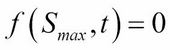
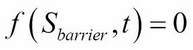
Let's take a look at an example of a down-and-out option. At any time during the life of the option, should the underlying asset price fall below a Sbarrier barrier price, the option is considered worthless. Since in the grid the finite difference scheme represents all the possible price points, we only need to consider nodes with the following price range:
We can then set up the boundary conditions as follows:
Let's create a class named FDCnDo that inherits from the FDCnEu class we discussed earlier. We can take into account the barrier price in the constructor method, while leaving the rest of the Crank-Nicolson implementation in the FDCnEu class unchanged:
"""
Price a down-and-out option by the Crank-Nicolson
method of finite differences.
"""
import numpy as np

from FDCnEu import FDCnEu


class FDCnDo(FDCnEu):

    def __init__(self, S0, K, r, T, sigma, Sbarrier, Smax, M, N,
                 is_call=True):
        super(FDCnDo, self).__init__(
            S0, K, r, T, sigma, Smax, M, N, is_call)
        self.dS = (Smax-Sbarrier)/float(self.M)
        self.boundary_conds = np.linspace(Sbarrier,
                                          Smax,
                                          self.M+1)
        self.i_values = self.boundary_conds/self.dS
Consider an example of a down-and-out option. The underlying stock price is $50 with a volatility of 40 percent. The strike price of the option is $50 with an expiration time of 5 months. The risk-free rate is 10 percent. The barrier price is $40.
We can price a call option and a put down-and-out option with Smax as 100, M as 120, and N as 500:
>>> from FDCnDo import FDCnDo
>>> option = FDCnDo(50, 50, 0.1, 5./12., 0.4, 40, 100, 120, 500)
>>> print option.price()
5.49156055293
>>> option = FDCnDo(50, 50, 0.1, 5./12., 0.4, 40, 100, 120, 500,
...                 False)
>>> print option.price()
0.541363502895
The prices of the down-and-out call and put options are $5.4916 and $0.5414 respectively.
So far, we have priced European options and exotic options. Due to the probability of an early exercise nature in American options, pricing such options is less straightforward. An iterative procedure is required in the implicit Crank-Nicolson method, where the payoffs from early exercises in the current period take into account the payoffs of an early exercise in the prior period. The Gauss-Siedel iterative method is proposed in the pricing of American options in the Crank-Nicolson method.
Remember in Chapter 2, The Importance of Linearity in Finance, we covered the Gauss-Siedel method of solving systems of linear equations in the form of ![]() . Here, the matrix A is decomposed into
. Here, the matrix A is decomposed into ![]() , where L is a lower triangular matrix and U is an upper triangular matrix. Let's take a look at an example of a 4 by 4 matrix A:
, where L is a lower triangular matrix and U is an upper triangular matrix. Let's take a look at an example of a 4 by 4 matrix A:

The solution is then obtained iteratively as follows:

We can adapt the Gauss-Siedel method to our Crank-Nicolson implementation as follows:
This equation satisfies the early exercise privilege equation:
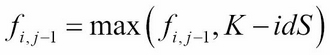
Let's create a class named FDCnAm that inherits from the FDCnEu class, which is the Crank-Nicolson method's counterpart for pricing European options. The _setup_coefficients_ method may be reused, while overriding all other methods for the inclusion of payoffs from an early exercise, if any:
""" Price an American option by the Crank-Nicolson method """
import numpy as np
import sys

from FDCnEu import FDCnEu


class FDCnAm(FDCnEu):

    def __init__(self, S0, K, r, T, sigma, Smax, M, N, omega, tol,
                 is_call=True):
        super(FDCnAm, self).__init__(
            S0, K, r, T, sigma, Smax, M, N, is_call)
        self.omega = omega
        self.tol = tol
        self.i_values = np.arange(self.M+1)
        self.j_values = np.arange(self.N+1)

    def _setup_boundary_conditions_(self):
        if self.is_call:
            self.payoffs = np.maximum(
                self.boundary_conds[1:self.M]-self.K, 0)
        else:
            self.payoffs = np.maximum(
                self.K-self.boundary_conds[1:self.M], 0)

        self.past_values = self.payoffs
        self.boundary_values = self.K *
                               np.exp(-self.r *
                                      self.dt *
                                      (self.N-self.j_values))

    def _traverse_grid_(self):
        """ Solve using linear systems of equations """
        aux = np.zeros(self.M-1)
        new_values = np.zeros(self.M-1)

        for j in reversed(range(self.N)):
            aux[0] = self.alpha[1]*(self.boundary_values[j] +
                                    self.boundary_values[j+1])
            rhs = np.dot(self.M2, self.past_values) + aux
            old_values = np.copy(self.past_values)
            error = sys.float_info.max

            while self.tol < error:
                new_values[0] =
                    max(self.payoffs[0],
                        old_values[0] +
                        self.omega/(1-self.beta[1]) *
                        (rhs[0] -
                         (1-self.beta[1])*old_values[0] +
                         (self.gamma[1]*old_values[1])))

                for k in range(self.M-2)[1:]:
                    new_values[k] =
                        max(self.payoffs[k],
                            old_values[k] +
                            self.omega/(1-self.beta[k+1]) *
                            (rhs[k] +
                             self.alpha[k+1]*new_values[k-1] -
                             (1-self.beta[k+1])*old_values[k] +
                             self.gamma[k+1]*old_values[k+1]))

                new_values[-1] =
                    max(self.payoffs[-1],
                        old_values[-1] +
                        self.omega/(1-self.beta[-2]) *
                        (rhs[-1] +
                         self.alpha[-2]*new_values[-2] -
                         (1-self.beta[-2])*old_values[-1]))

                error = np.linalg.norm(new_values - old_values)
                old_values = np.copy(new_values)

            self.past_values = np.copy(new_values)

        self.values = np.concatenate(([self.boundary_values[0]],
                                      new_values,
                                      [0]))

    def _interpolate_(self):
        # Use linear interpolation on final values as 1D array
        return np.interp(self.S0,
                         self.boundary_conds,
                         self.values)
The tolerance parameter is used in the Gauss-Siedel method as the convergence criterion. The omega is the over-relaxation parameter. Higher omega values give faster convergence, but this also comes with higher possibilities of the algorithm not converging.
Let's price an American call-and-put option with an underlying asset price of $50 and volatility of 40 percent, a strike price of $50, a risk-free rate of 10 percent, and an expiration date of 5 months. We choose a Smax value of 100, M as 100, N as 42, an omega parameter value of 1.2, and a tolerance value of 0.001:
>>> from FDCnDo import FDCnDo
>>> option = FDCnAm(50, 50, 0.1, 5./12., 0.4, 100, 100,
...                 42, 1.2, 0.001)
>>> print option.price()
6.10868281539
>>> option = FDCnAm(50, 50, 0.1, 5./12., 0.4, 100, 100,
...                 42, 1.2, 0.001, False)
>>> print option.price()
4.27776422938
The prices of the call-and-put American stock options by the Crank-Nicolson method are $6.109 and $4.2778 respectively.