
Chapter 5 Flex, sag and wobble: Stiffness-limited design
- 5.1 Introduction and synopsis 82
- 5.2 Standard solutions to elastic problems 82
- 5.3 Material indices for elastic design 90
- 5.4 Plotting limits and indices on charts 97
- 5.5 Case studies 100
- 5.6 Summary and conclusions 107
- 5.7 Further reading 108
- 5.8 Exercises 108
- 5.9 Exploring design with CES 109
- 5.10 Exploring the science with CES Elements 110
A few years back, with the millennium approaching, countries and cites around the world turned their minds to iconic building projects. In Britain there were several. One was—well, is—a new pedestrian bridge spanning the river Thames, linking St Paul’s Cathedral to the Museum of Modern Art facing it across the river. The design was—oops, is—daring: a suspension bridge with suspension cables that barely rise above the level of the deck instead of the usual great upward sweep. The result was visually striking: a sleek, slender, span like a ‘shaft of light’ (the architect’s words). Just one problem: it wasn’t stiff enough. The bridge opened but when people walked on it, it swayed and wobbled so alarmingly that it was promptly closed. A year and $5 000 000 later it reopened, much modified, and now it is fine.
A pole vaulter—the pole stores elastic energy. (Image courtesy of Gill Athletics, 2808 Gemini Court, Champaign, IL 61822-9648, USA)

5.1 Introduction and synopsis
A few years back, with the millennium approaching, countries and cites around the world turned their minds to iconic building projects. In Britain there were several. One was—well, is—a new pedestrian bridge spanning the river Thames, linking St Paul’s Cathedral to the Museum of Modern Art facing it across the river. The design was—oops, is—daring: a suspension bridge with suspension cables that barely rise above the level of the deck instead of the usual great upward sweep. The result was visually striking: a sleek, slender, span like a ‘shaft of light’ (the architect’s words). Just one problem: it wasn’t stiff enough. The bridge opened but when people walked on it, it swayed and wobbled so alarmingly that it was promptly closed. A year and $5 000 000 later it reopened, much modified, and now it is fine.
The first thing you tend to think of with structures, bridges included, is strength: they must not fall down. Stiffness, often, is taken for granted. But, as the bridge story relates, that can be a mistake—stiffness is important. Here we explore stiffness-limited design and the choice of materials to achieve it. This involves the modeling of material response in a given application. The models can be simple because the selection criteria that emerge are insensitive to the details of shape and loading. The key steps are those of identifying the constraints that the material must meet and the objective by which the excellence of choice will be measured.
We saw at the beginning of Chapter 4 that there are certain common modes of loading: tension, compression, bending and torsion. The loading on any real component can be decomposed into some combination of these. So it makes sense to have a catalog of solutions for the standard modes, relating the component response to the loading. In this chapter, the response is elastic deflection; in later chapters it will be yielding or fracture. You don’t need to know how to derive all of these—they are standard results—but you do need to know where to find them. You will find the most useful of them here; the sources listed under ‘Further reading’ give more. And, most important, you need to know how to use them. That needs practice—you get some of that here too.
The first section of this chapter, then, is about standard solutions to elastic problems. The second is about their use to derive material limits and indices. The third explains how to plot them onto material property charts. The last illustrates their use via case studies.
5.2 Standard solutions to elastic problems
Modeling is a key part of design. In the early, conceptual stage, approximate models establish whether a concept will work at all and identify the combination of material properties that maximise performance. At the embodiment stage, more accurate modeling brackets values for the design parameters: forces, displacements, velocities, heat fluxes and component dimensions. And in the final stage, modeling gives precise values for stresses, strains and failure probabilities in key components allowing optimised material selection and sizing.
Many common geometries and load patterns have been modeled already. A component can often be modeled approximately by idealising it as one of these. There is no need to reanalyse the beam or the column or the pressure vessel; their behaviour under all common types of loading has already been analysed. The important thing is to know that the results exist, where to find them and how to use them.
This section is a bit tedious (as books on the strength of materials tend to be) but the results are really useful. Here they are listed, defining the quantities that enter and the components to which they apply.
Elastic extension or compression
A tensile or compressive stress σ = F/A applied axially to a tie or strut of length Lo and constant cross-section area A suffers a strain ε = σ/E. The strain ε is related to the extension δ by ε = δ/Lo (Figure 5.1(a)). Thus, the relation between the load F and deflection δ is
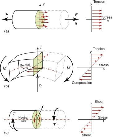
Figure 5.1 (a) A tie with a cross-section A loaded in tension. Its stiffness is S = F/δ. (b) A beam of rectangular cross-section loaded in bending. The stress σ varies linearly from tension to compression, changing sign at the neutral axis, resulting in a bending moment M. (c) A shaft of circular cross-section loaded in torsion.

Note that the shape of the cross-section area does not matter because the stress is uniform over the section.
Elastic bending of beams
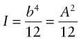
When a beam is loaded by a bending moment M, its initially straight axis is deformed to a curvature κ (Figure 5.1(b))

where u is the displacement parallel to the y-axis. The curvature generates a linear variation of axial strain ε (and thus stress σ) across the section, with tension on one side and compression on the other—the position of zero stress being the neutral axis. The stress increases with distance y from the neutral axis. Material is more effective at resisting bending the farther it is from that axis, so the shape of the cross-section is important. Elastic beam theory gives the stress σ caused by a moment M in a beam made of material of Young’s modulus E, as


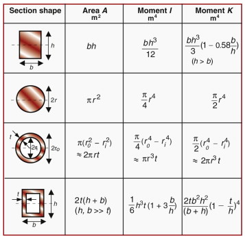
where I is the second moment of area, defined as
The distance y is measured vertically from the neutral axis and b(y) is the width of the section at y. The moment I characterises the resistance of the section to bending—it includes the effect of both size and shape. Examples for four common sections are listed in Figure 5.2 with expressions for the cross-section area A and the second moment of area, I.
Example 5.1
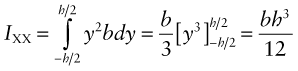
- (a) A beam has a rectangular cross with height h and width b. Show that the second moment of area is I = bh3/12.
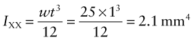
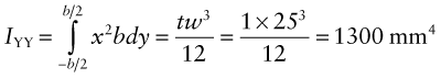
- (b) A steel ruler is 300 mm long with a width w = 25 mm and a thickness t = 1 mm. Calculate the second moments of area IXX and IYY.
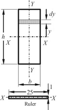
- (a) For bending about the X-X axis, consider a narrow horizontal strip of height dy and width b. Inserting this into (5.4) gives:
- (b) For the steel ruler, bending about the (flexible) X-X axis:
whereas for bending about the (stiff) Y-Y axis:
IYY is more than 600 times greater than IXX, because the material of the ruler is located close to the X-X axis but (on average) farther away from the Y-Y axis.
Moments of inertia for complex sections can be calculated by superimposing the results for simple shapes like the rectangle (though sometimes you may need to use the ‘parallel axis theorem’—see books on mechanics of structures).
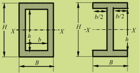
For both the rectangular hollow section and the I-section shown, IXX can be calculated by subtracting IXX for a small rectangle (b × h) from the value of IXX for the large rectangle (B × H), giving:
Moments of area are tabulated in books for standard cases, and in tables of structural sections for commercially available section shapes.
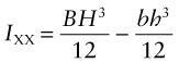
The ratio of moment to curvature, M/κ, is called the flexural rigidity, EI. Figure 5.3 shows three possible distributions of load F, each creating a distribution of moment M(x). The maximum deflection, δ, is found by integrating equation (5.3) twice for a particular M(x). For a beam of length L with a transverse load F, the stiffness is
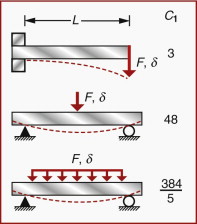
Figure 5.3 Elastic deflection of beams. The deflection δ of a span L under a force F depends on the flexural stiffness EI of the cross-section and the way the force is distributed. The constant C1 is defined in equation (5.5).
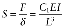
The result is the same for all simple distributions of load; the only thing that depends on the distribution is the value of the constant C1; the figure lists values for the three distributions. We will find in Section 5.3 that the best choice of material is independent of the value of C1 with the happy result that the best choice for a complex distribution of loads is the same as that for a simple one.
Example 5.2
- (a) The ruler in Example 5.1 is made of stainless steel with Young’s modulus of 200 GPa. A student supports the ruler as a horizontal cantilever, with 250 mm protruding from the edge of a table and hangs a weight of 10 N on the free end. Calculate the vertical deflection of the free end if the ruler is mounted with: (i) the X-X axis horizontal; (ii) the Y-Y axis horizontal. (Ignore the deflection caused by the self-weight of the ruler.)
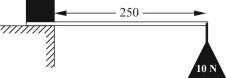
Use equation (5.5) with C1 = 3 (from Figure 5.3), and use IXX and IYY from Example 5.1.
This shows the dramatic benefit of locating the material of a beam as far as possible from the bending axis, so as to maximise the second moment of area. Consequently ‘I-sections’ are often used for structural girders.
- (b) A new ruler is to be made from polystyrene, with Young’s modulus of 2 GPa. Its length and width are to be the same as the stainless steel ruler, but its thickness can be changed by the designer. The polystyrene ruler is to be mounted with its X-X axis horizontal and its deflection must not be any greater than that of the stainless steel ruler under the 10 N end load. Calculate the thickness needed to achieve this. Compare the masses of the two rulers. (The densities of stainless steel and polystyrene are 7800 kg/m3 and 1040 kg/m3.)
Answer. Using the same equations,![]()
The thickness can be found from ![]() :
:![]() .
.
The masses are: mSS = 7800 × 0.3 × 0.025 × 0.001 = 59 g and mPS = 1040 × 0.3 × 0.025 × 0.0046 = 36 g. Despite its much lower density, the polystyrene ruler is only 40% lighter than the stainless steel one, because of its much greater thickness.
Torsion of shafts
A torque, T, applied to the ends of an isotropic bar of a uniform section generates a shear stress τ (Figures 5.1(c) and 5.4). For circular sections, the shear stress varies with radial distance r from the axis of symmetry is
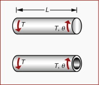
Figure 5.4 Elastic torsion of circular shafts. The stress in the shaft and the twist per unit length depend on the torque T and the torsional rigidity GK.

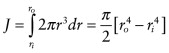
where K measures the resistance of the section to twisting (the torsional equivalent to I, for bending). K is easiest to calculate for circular sections, when it is equal to the polar second moment of area:
where r is measured radially from the centre of the circular section. For non-circular sections, K is less than J. Figure 5.2 gives expressions for K for four standard shapes.
The shear stress acts in the plane normal to the axis of the bar. It causes the bar, with length L, to twist through an angle θ. The twist per unit length, θ/L, is related to the shear stress and the torque by
where G is the shear modulus. The ratio of torque to twist, T/θ, per unit length, is equal to GK, called the torsional rigidity.
Example 5.3
- (a) Derive an expression for the polar second moment of area of a tube having a hollow circular section with inner radius ri and outer radius ro.
- (b) A brass rod with shear modulus 40 GPa, length 200 mm, and having a solid circular cross-section with diameter 10 mm, is twisted with a torque of 10 Nm. What is the angle of twist?
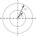
- (a) Applying equation (5.7):
- (b) For a rod with a solid circular section of radius R = 5 mm,
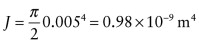 . So the angle of twist is given by:
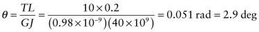
Buckling of columns and plates
If sufficiently slender, an elastic column or plate, loaded in compression, fails by elastic buckling at a critical load, Fcrit. Beam theory shows that the critical buckling load depends on the length L and flexural rigidity, EI:
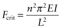
where n is a constant that depends on the end constraints: clamped, or free to rotate, or free also to translate (Figure 5.5). The value of n is just the number of half-wavelengths of the buckled shape (the half-wavelength is the distance between inflection points).
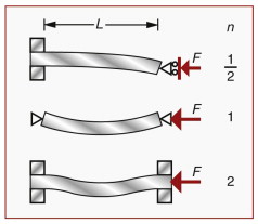
Figure 5.5 The buckling load of a column of length L depends on the flexural rigidity EI and on the end constraints; three are shown here, together with the value of n.
Some of the great engineering disasters have been caused by buckling. It can occur without warning and slight misalignment is enough to reduce the load at which it happens. When dealing with compressive loads on columns or in-plane compression of plates it is advisable to check that you are well away from the buckling load.
Vibrating beams and plates
Any undamped system vibrating at one of its natural frequencies can be reduced to the simple problem of a mass m attached to a spring of stiffness k—the restoring force per unit displacement. The lowest natural frequency of such a system is
Different geometries require appropriate estimates of the effective k and m—often these can be estimated with sufficient accuracy by approximate modeling. The higher natural frequencies of rods and beams are simple multiples of the lowest.
Figure 5.6 shows the lowest natural frequencies of the flexural modes of uniform beams or plates of length L with various end constraints. The spring stiffness, k, is that for bending, given by equation (5.5), so the natural frequencies can be written:
where C2, listed in the figure, depends on the end constraints and mo is the mass of the beam per unit length. The mass per unit length is just the area times the density, Aρ, so the natural frequency becomes
5.3 Material indices for elastic design
We can now start to implement the steps outlined in Chapter 3 and summarised in Figure 3.6:
- Translation.
- Screening, based on constraints.
- Ranking, based on objectives.
- Documentation, to give greater depth.
The first two were fully described in Chapter 3. The third—ranking based on objectives—requires simple modeling to identify the material index.
An objective, remember, is a criterion of excellence for the design as a whole, something to be minimised (like cost, weight or volume) or maximised (like energy storage). Here we explore those for elastic design.
Minimising weight: a light, stiff tie-rod
Think first of choosing a material for a cylindrical tie-rod like one of those in the cover picture of Chapter 4. Its length Lo is specified and it must carry a tensile force F without extending elastically by more than δ. Its stiffness must be at least S* = F/δ (Figure 5.7(a)). This is a load-carrying component, so it will need to have some toughness. The objective is to make it as light as possible. The cross-section area A is free. The design requirements, translated, are listed in Table 5.1.
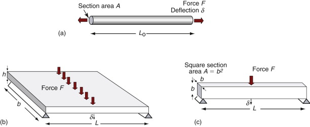
Figure 5.7 (a) A tie with cross-section area A, loaded in tension. Its stiffness is S = F/δ where F is the load and δ is the extension. (b) A panel loaded in bending. Its stiffness is S = F/δ, where F is the total load and δ is the bending deflection. (c) A beam of square section, loaded in bending. Its stiffness is S = F/δ, where F is the load and δ is the bending deflection.
Table 5.1 Design requirements for the light, stiff tie
|
We first seek an equation that describes the quantity to be maximised or minimised, here the mass m of the tie. This equation, called the objective function, is
where A is the area of the cross-section and ρ is the density of the material of which it is made. We can reduce the mass by reducing the cross-section, but there is a constraint: the section area A must be sufficient to provide a stiffness of S*, which, for a tie, is given by equation (5.2):

If the material has a low modulus, a large A is needed to give the necessary stiffness; if E is high, a smaller A is needed. But which gives the lower mass? To find out, we eliminate the free variable A between these two equations, giving
Both S* and Lo are specified. The lightest tie that will provide a stiffness S* is that made of the material with the smallest value of ρ/E. We could define this as the material index of the problem, seeking the material with a minimum value, but it is more usual to express indices in a form for which a maximum is sought. We therefore invert the material properties in equation (5.15) and define the material index Mt (subscript ‘t’ for tie) as:

It is called the specific stiffness. Materials with a high value of Mt are the best choice, provided that they also meet any other constraints of the design, in this case the need for some toughness.
The mode of loading that most commonly dominates in engineering is not tension, but bending—think of floor joists, of wing spars, of golf club shafts. The index for bending differs from that for tension, and this (significantly) changes the optimal choice of material. We start by modeling panels and beams, specifying stiffness and seeking to minimise weight.
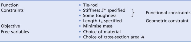
Minimising weight: a light, stiff panel
A panel is a flat slab, like a table top. Its length L and width b are specified but its thickness h is free. It is loaded in bending by a central load F (Figure 5.7(b)). The stiffness constraint requires that it must not deflect more than δ under the load F and the objective is again to make the panel as light as possible. Table 5.2 summarises the design requirements.
Table 5.2 Design requirements for the light, stiff panel
| Function | • Panel | |
| Constraints | Functional constraint | |
| Geometric constraint | ||
| Objective | • Minimise mass | |
| Free variables |
The objective function for the mass of the panel is the same as that for the tie:
Its bending stiffness S is given by equation (5.5). It must be at least:

The second moment of area, I, for a rectangular section (Table 5.2) is

The stiffness S*, the length L and the width b are specified; only the thickness h is free. We can reduce the mass by reducing h, but only so far that the stiffness constraint is still met. Using the last two equations to eliminate h in the objective function for the mass gives
The quantities S*, L, b and C1 are all specified; the only freedom of choice left is that of the material. The best materials for a light, stiff panel are those with the smallest values of ρ/E1/3 (again, so long as they meet any other constraints). As before, we will invert this, seeking instead large values of the material index Mp for the panel:

This doesn’t look much different from the previous index, E/ρ, but it is. It leads to a different choice of material, as we shall see in a moment. For now, note the procedure. The length of the panel was specified but we were free to vary the section area. The objective is to minimise its mass, m. Use the stiffness constraint to eliminate the free variable, here h. Then read off the combination of material properties that appears in the objective function—the equation for the mass. It is the index for the problem.
It sounds easy, and it is—so long as you are clear from the start what the constraints are, what you are trying to maximise or minimise and which parameters are specified and which are free.
Now we look at another bending problem, in which the freedom to choose shape is rather greater than for the panel.
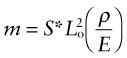
Minimising weight: a light, stiff beam
Beams come in many shapes: solid rectangles, cylindrical tubes, I-beams and more. Some of these have too many free geometric variables to apply the previous method directly. However, if we constrain the shape to be self-similar (such that all dimensions change in proportion as we vary the overall size), the problem becomes tractable again. We therefore consider beams in two stages: first, to identify the optimum materials for a light, stiff beam of a prescribed simple shape (such as a square section); then, second, we explore how much lighter it could be made, for the same stiffness, by using a more efficient shape.
Consider a beam of square section A = b × b that may vary in size but with the square shape retained. It is loaded in bending over a span of fixed length L with a central load F (Figure 5.7(c)). The stiffness constraint is again that it must not deflect more than δ under the load F, with the objective that the beam should again be as light as possible. Table 5.3 summarises the design requirements.
Table 5.3 Design requirements for the light, stiff beam
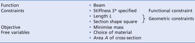
|
Proceeding as before, the objective function for the mass is:
The beam bending stiffness S (equation (5.5)) is

The second moment of area, I, for a square section beam is
For a given length L, the stiffness S* is achieved by adjusting the size of the square section. Now eliminating b (or A) in the objective function for the mass gives
The quantities S*, L and C1 are all specified—the best materials for a light, stiff beam are those with the smallest values of ρ/E1/2. Inverting this, we require large values of the material index Mb for the beam:

This analysis was for a square beam, but the result in fact holds for any shape, so long as the shape is held constant. This is a consequence of equation (5.24)—for a given shape, the second moment of area I can always be expressed as a constant times A2, so changing the shape just changes the constant C1 in equation (5.25), not the resulting index.
As noted earlier, real beams have section shapes that improve their efficiency in bending, requiring less material to get the same stiffness. By shaping the cross-section it is possible to increase I without changing A. This is achieved by locating the material of the beam as far from the neutral axis as possible, as in thin-walled tubes or I-beams. Some materials are more amenable than others to being made into efficient shapes. Comparing materials on the basis of the index in equation (5.26) therefore requires some caution—materials with lower values of the index may ‘catch up’ by being made into more efficient shapes. So we need to get an idea of the effect of shape on bending performance.
Figure 5.8 shows a solid square beam, of cross-section area A. If we turned the same area into a tube, as shown in the left of the figure, the mass of the beam is unchanged (equation (5.22)). The second moment of area, I, however, is now much greater—and so is the stiffness (equation (5.23)). We define the ratio of I for the shaped section to that for a solid square section with the same area (and thus mass) as the shape factor Φ. The more slender the shape the larger is Φ, but there is a limit—make it too thin and the tube will buckle—so there is a maximum shape factor for each material that depends on its properties. Table 5.4 lists some typical values.
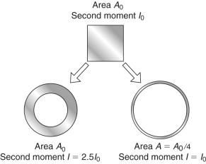
Figure 5.8 The effect of section shape on bending stiffness EI: a square-section beam compared, left, with a tube of the same area (but 2.5 times stiffer) and, right, a tube with the same stiffness (but four times lighter).
Table 5.4 The effect of shaping on stiffness and mass of beams in different structural materials
| Material | Typical maximum shape factor (stiffness relative to that of a solid square beam) | Typical mass ratio by shaping (relative to that of a solid square beam) |
|---|---|---|
| Steels | 64 | 1/8 |
| Al alloys | 49 | 1/7 |
| Composites (GFRP, CFRP) | 36 | 1/6 |
| Wood | 9 | 1/3 |
Shaping is also used to make structures lighter: it is a way to get the same stiffness with less material (Figure 5.8, right). The mass ratio is given by the reciprocal of the square root of the maximum shape factor, Φ−1/2 (because C1, which is proportional to the shape factor, appears as (C1)−1/2 in equation (5.25)). Table 5.4 lists the factor by which a beam can be made lighter, for the same stiffness, by shaping. Metals and composites can all be improved significantly (though the metals do a little better), but wood has more limited potential because it is more difficult to shape it into efficient, thin-walled shapes. So, when comparing materials for light, stiff beams using the index in equation (5.26), the performance of wood is not as good as it looks because other materials can be made into more efficient shapes. As we will see, composites (particularly CFRP) have very high values of all three indices Mt, Mp and Mb, but this advantage relative to metals is reduced a little by the effect of shape.
Shaping offers exactly the same benefits under torsional loading—a tube of the same mass has a greater resistance to twisting (or, alternatively, a lighter tube can do the same job as a solid circular rod). The following example illustrates the effect.
Example 5.4
The brass rod in Example 5.3 is formed into a hollow tube with an outer radius of 25 mm, and the same length, using the same amount of material. It is twisted with the same torque. What is its angle of twist? Compare its torsional stiffness with the solid rod in Example 5.3.
Answer. To have the same amount of material, the cross-section area of the tube ![]() must equal that of the solid bar πR2. Therefore the inner radius of the tube must be
must equal that of the solid bar πR2. Therefore the inner radius of the tube must be
(i.e. a wall thickness of 1 mm). The polar moment of area of the tube is then:
and the angle of twist is

This compares to 2.9 deg for the solid shaft in Example 5.3. Therefore the hollow shaft, which has the same mass as the solid one, has about 11 times the torsional stiffness (T/θ).
Minimising material cost
When the objective is to minimise cost rather than weight, the indices change. If the material price is Cm $/kg, the cost of the material to make a component of mass m is just mCm. The objective function for the material cost C of the tie, panel or beam then becomes
Proceeding as in the three previous examples then leads to indices that are just those of equations (5.16), (5.21) and (5.26), with ρ replaced by Cmρ.
The material cost is only part of the cost of a shaped component; there is also the manufacturing cost—the cost to shape, join and finish it. We leave these to a later chapter.
5.4 Plotting limits and indices on charts
Screening: attribute limits on charts
Any design imposes certain non-negotiable demands (constraints) on the material of which it is made. These limits can be plotted as horizontal or vertical lines on material property charts, as illustrated in Figure 5.9, which shows a schematic of the E–Relative cost chart of Figure 4.7. We suppose that the design imposes limits on these of E > 10 GPa and Relative cost < 3, shown in the figure. All materials in the window defined by the limits, labeled ‘Search region’, meet both constraints.
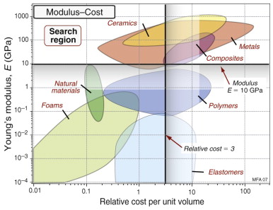
Figure 5.9 A schematic E–Relative cost chart showing a lower limit for E and an upper one for Relative cost.
Later chapters of this book show charts for many other properties. They allow limits to be imposed on other properties.
Ranking: indices on charts
The next step is to seek, from the subset of materials that meet the property limits, those that maximise the performance of the component. We will use the design of light, stiff components as examples; the other material indices are used in a similar way.
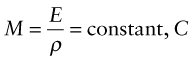
Figure 5.10 shows a schematic of the E–ρ chart of Figure 4.6. The logarithmic scales allow all three of the indices E/ρ, E1/3/ρ and E1/2/ρ, derived in the last section, to be plotted onto it. Consider the condition
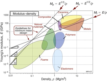
Figure 5.10 A schematic E–ρ chart showing guidelines for three material indices for stiff, lightweight structures.
that is, a particular value of the specific stiffness. Taking logs,
This is the equation of a straight line of slope 1 on a plot of log(E) against log(ρ), as shown in the figure. Similarly, the condition
becomes, on taking logs,
This is another straight line, this time with a slope of 3, also shown. And by inspection, the third index E1/2/ρ will plot as a line of slope 2. We refer to these lines as selection guidelines. They give the slope of the family of parallel lines belonging to that index.
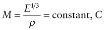
It is now easy to read off the subset of materials that maximise performance for each loading geometry. For example, all the materials that lie on a line of constant M = E1/3/ρ perform equally well as a light, stiff panel; those above the line perform better, those below less well. Figure 5.11 shows a grid of lines corresponding to values of M = E1/3/ρ from M = 0.22 to M = 4.6 in units of GPa1/3/(Mg/m3). A material with M = 3 in these units gives a panel that has one-tenth the weight of one with M = 0.3. The case studies in the next section give practical examples.
Computer-aided selection
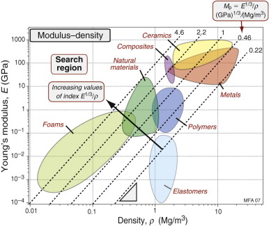
The charts give an overview, but the number of materials that can be shown on any one of them is obviously limited. Selection using them is practical when there are very few constraints, but when there are many—as there usually are—checking that a given material meets them all is cumbersome. Both problems are overcome by a computer implementation of the method.
The CES material and process selection software1 is an example of such an implementation. Its database contains records for materials, organised in the hierarchical manner shown in Figure 2.3 in Chapter 2. Each record contains property data for a material, each property stored as a range spanning its typical (or, often, permitted) values. It also contains limited documentation in the form of text, images and references to sources of information about the material. The data are interrogated by a search engine that offers the search interfaces shown schematically in Figure 5.12. On the left is a simple query interface for screening on single attributes. The desired upper or lower limits for constrained properties are entered; the search engine rejects all materials with attributes that lie outside the limits. In the centre is shown a second way of interrogating the data: a bar chart, constructed by the software, for any numeric property in the database. It, and the bubble chart shown on the right, are ways both of applying constraints and of ranking. For screening, a selection line or box is superimposed on the charts with edges that lie at the constrained values of the property (bar chart) or properties (bubble chart). This eliminates the materials in the shaded areas and retains the materials that meet the constraints. If, instead, ranking is sought (having already applied all necessary constraints) an index-line like that shown in Figure 5.11 is positioned so that a small number—say, 10—of materials are left in the selected area; these are the top-ranked candidates. The software delivers a list of the top-ranked materials that meet all the constraints.
5.5 Case studies
Here we have case studies using the two charts of Chapter 4. They are deliberately simplified to avoid obscuring the method under layers of detail. In most cases little is lost by this: the best choice of material for the simple example is the same as that for the more complex.
Light levers for corkscrews
The lever of the corkscrew (Figure 5.13) is loaded in bending: the force F creates a bending moment M = FL. The lever needs to be stiff enough that the bending displacement, δ, when extracting a cork, is acceptably small. If the corkscrew is intended for travelers, it should also be light. The section is rectangular. We make the assumption of self-similarity, meaning that we are free to change the scale of the section but not its shape. The material index we want was derived earlier as equation (5.26). It is that for a light, stiff beam:
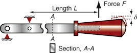
Figure 5.13 The corkscrew lever from Chapter 3. It must be adequately stiff and, for traveling, as light as possible.

where E is Young’s modulus and ρ is the density. There are other obvious constraints. Corkscrews get dropped and must survive impacts of other kinds, so brittle materials like glass or ceramic are unacceptable. Given these requirements, summarised in Table 5.5, what materials would you choose?
Table 5.5 Design requirements for the corkscrew lever
| Function | • Lightweight lever, meaning light, stiff beam |
| Constraints | |
| Objective | • Minimise mass |
| Free variables |
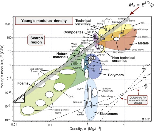
Figure 5.14 shows the appropriate chart: that in which Young’s modulus, E, is plotted against density, ρ. The selection line for the index M has a slope of 2, as explained in Section 5.3; it is positioned so that a small group of materials is left above it. They are the materials with the largest values of M, and it is these that are the best choice, provided they satisfy the other constraints. Three classes of materials lie above the line: woods, carbon-fiber reinforced polymers (CFRPs) and a number of ceramics. Ceramics are brittle and expensive, ruling them out. The recommendation is clear. Make your the lever out of wood or—better—out of CFRP.
Cost: structural materials for buildings
The most expensive thing that most people ever buy is the house they live in. Roughly half the cost of a house is the cost of the materials of which it is made, and these are used in large quantities (family house: around 200 tonnes; large apartment block: around 20 000 tonnes). The materials are used in three ways: structurally to hold the building up; as cladding, to keep the weather out; and as ‘internals’, to insulate against heat and sound, and to provide comfort and decoration.
Consider the selection of materials for the structure (Figure 5.15). They must be stiff, strong and cheap: stiff, so that the building does not flex too much under wind loads or internal loading; strong, so that there is no risk of it collapsing; and cheap, because such a lot of material is used. The structural frame of a building is rarely exposed to the environment, and is not, in general, visible, so criteria of corrosion resistance or appearance are not important here. The design goal is simple: stiffness and strength at minimum cost. To be more specific: consider the selection of material for floor joists, focusing on stiffness. Table 5.6 summarises the requirements.
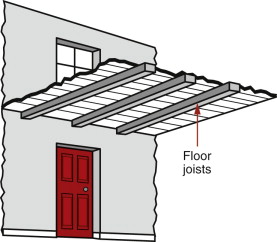
Figure 5.15 The materials of a building are chosen to perform three different roles. Those for the structure are chosen to carry loads. Those for the cladding provide protection from the environment. Those for the interior control heat, light and sound. Here we explore structural materials.
Table 5.6 Design requirements for floor beams
| Function | • Floor beam |
| Constraints | |
| Objective | • Minimise material cost |
| Free variables |
The material index for a stiff beam of minimum mass, m, was developed earlier. The cost C of the beam is just its mass, m, times the cost per kg, Cm, of the material of which it is made:
Proceeding as in Section 5.3, we find the index for a stiff beam of minimum cost to be:

Figure 5.16 shows the relevant chart: modulus E against relative cost per unit volume, Cm ρ (the chart uses a relative cost Cv,R, defined in Chapter 4, in place of Cm but this makes no difference to the selection). The shaded band has the appropriate slope for M; it isolates concrete, stone, brick, woods, cast irons and carbon steels.
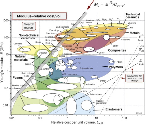
Figure 5.16 The selection of materials for stiff floor beams. The objective is to make them as cheap as possible while meeting a stiffness constraint.
Concrete, stone and brick have strength only in compression; the form of the building must use them in this way (walls, columns, arches). Wood, steel and reinforced concrete have strength both in tension and compression, and steel, additionally, can be given efficient shapes (I-sections, box sections, tubes) that can carry bending and tensile loads as well as compression, allowing greater freedom of the form of the building.
Cushions and padding: the modulus of foams
One way of manipulating the modulus is to make a material into a foam. Figure 4.23 showed an idealised foam structure: a network of struts of length L and thickness t, connected at their mid-span to neighbouring cells. Cellular solids like this one are characterised by their relative density, which for the structure shown here (with t ≪ L) is
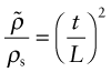
where ![]() is the density of the foam and ρs is the density of the solid of which it is made.
is the density of the foam and ρs is the density of the solid of which it is made.
If a compressive stress σ is applied to a block of foam containing many cells, it is transmitted through the foam as forces F pushing on edges that lie parallel to the direction of σ. The area of one cell face is L2 so the force on one strut is F = σL2. This force bends the cell edge to which it connects, as on the right of Figure 4.23. Thus, the cell edge is just a beam, built-in at both ends, carrying a central force F. The bending deflection is given by equation (5.5):

where Es is the modulus of the solid of which the foam is made and I = t4/12 is the second moment of area of the cell edge of square cross-section, t × t. The compressive strain suffered by the cell as a whole is then ε = 2δ/L. Assembling these results gives the modulus ![]() of the foam as
of the foam as
Since ![]() when
when ![]() , the constant of proportionality is 1, giving the result plotted earlier in Figure 4.24.
, the constant of proportionality is 1, giving the result plotted earlier in Figure 4.24.
Vibration: avoiding resonance when changing material
Vibration, as the story at the start of this chapter relates, can be a big problem. Bridges are designed with sufficient stiffness to prevent wind-loads exciting their natural vibration frequencies (one, the Tacoma Straits bridge in the state of Washington, wasn’t; its oscillations destroyed it). Auto-makers invest massively in computer simulation of new models to be sure that door and roof panels don’t start thumping because the engine vibration hits a natural frequency. Even musical instruments, which rely on exciting natural frequencies, have problems with ‘rogue’ tones: notes that excite frequencies you didn’t want as well as those you did.
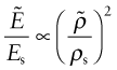
Suppose you redesign your bridge, or car, or cello and, in a creative moment, decide to make it out of a new material. What will it do to the natural frequencies? Simple. Natural frequencies, f, as explained in Section 5.2, are proportional to ![]() . If the old material has a modulus Eo and density ρo and the new one has En, ρn, the change in frequency, Δf
. If the old material has a modulus Eo and density ρo and the new one has En, ρn, the change in frequency, Δf
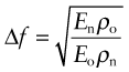
Provided this shift still leaves natural frequencies remote from those of the excitation, all is well. But if this is not so, a rethink would be prudent.
Bendy design: part-stiff, part-flexible structures
The examples thus far aimed at the design of components that did not bend too much—that is, they met a stiffness constraint. Elasticity can be used in another way: to design components that are strong but not stiff, arranging that they bend easily in a certain direction. Think, for instance, of a windscreen wiper blade. The frame to which the rubber squeegees are attached must adapt to the changing profile of the windscreen as it sweeps across it. It does so by flexing, maintaining an even pressure on the blades. This is a deliberately bendy structure.
Figure 5.17 shows two ways of making a spring-loaded plunger. The one on the left with a plunger and a spring involves sliding surfaces. The one on the right has none: it uses elastic bending to both locate and guide the plunger and to give the restoring force provided by the spring in the first design.
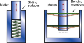
Exploiting elasticity in this way has many attractions. There is no friction, no wear, no need for lubrication, no precise clearances between moving parts. And in design with polymers there is another bonus; since there are no sliding surfaces it is often possible to mould the entire device as a single unit, reducing the part-count and doing away with the need for assembly. Reducing part-count is music to the ears of production engineers: it is cost-effective.
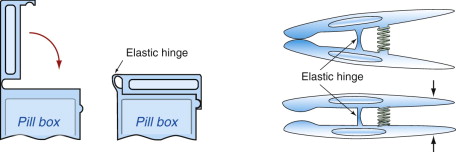
Figure 5.18 shows examples you will recognize: the ‘living hinge’ used on toothpaste tubes, moulded plastic boxes, clips and clothes pegs. Here the function of a rotational hinge is replaced by an elastic connecting strip, wide but thin. The width gives lateral registration; the thinness allows easy flexure. The traditional three-part hinge has been reduced to a single moulding.
There is much scope for imaginative design here. Figure 5.19 shows three section shapes, each allowing one or more degrees of elastic freedom, while retaining stiffness and strength in the other directions. By incorporating these into structures, parts can be allowed to move relative to the rest in controlled ways.
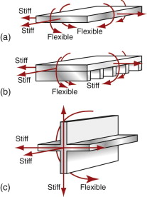
Figure 5.19 The flexural degrees of freedom of three alternative section shapes. (a) Thin plates are flexible about any axis in the plane of the plate, but are otherwise stiff. (b) Ribbed plates are flexible about one in-plane axis but not in others. (c) Cruciform beams are stiff in bending but can be twisted easily.
How do we choose materials for such elastic mechanisms? It involves a balance between stiffness and strength. Strength keeps appearing here—that means waiting until Chapter 7 for a full answer.
5.6 Summary and conclusions
Adequate stiffness is central to the design of structures that are deflection limited. The wing spar of an aircraft is an example: too much deflection compromises aerodynamic performance. Sports equipment is another: the feel of golf clubs, tennis rackets, skis and snowboards has much to do with stiffness. The sudden buckling of a drinking straw when you bend it is a stiffness-related problem—one that occurs, more disastrously, in larger structures. And when, as the turbine of an aircraft revs up, it passes through a speed at which vibration suddenly peaks, the cause is resonance linked to the stiffness of the turbine blades. Stiffness is influenced by the size and shape of the cross-section and the material of which it is made. The property that matters here is the elastic modulus E.
In selecting materials, adequate stiffness is frequently a constraint. This chapter explained how to meet it for various modes of loading and for differing objectives: minimising mass, or volume or cost. Simple modeling delivers expressions for the objective: for the mass, or for the material cost. These expressions contain material properties, either singly or in combination. It is these that we call the material index. Material indices measure the excellence of a material in a given application. They are used to rank materials that meet the other constraints.
Stiffness is useful, but lack of stiffness can be useful too. The ability to bend or twist allows elastic mechanisms: single components that behave as if they had moving parts with bearings. Elastic mechanisms have limitations, but—where practical—they require no assembly, they have no maintenance requirements and they are cheap.
The chapter ended by illustrating how indices are plotted onto material property charts to find the best selection. The method is a general one that we apply in later chapters to strength thermal, electrical, magnetic and optical properties.
Ashby M.F. Materials Selection in Mechanical Design 3rd ed. 2005 Butterworth-Heinemann Oxford, UK Chapter 4. ISBN 0-7506-6168-2. (A more advanced text that develops the ideas presented here, including a much fuller discussion of shape factors and an expanded catalog of simple solutions to standard problems.)
Gere J.M. Mechanics of Materials 6th ed. 2006 Thompson Publishing Toronto, Canada ISBN 0-534-41793-0. (An intermediate level text on statics of structures by one of the fathers of the field; his books with Timoshenko introduced an entire generation to the subject.)
Hosford W.F. Mechanical Behavior of Materials 2005 Cambridge University Press Cambridge, UK ISBN 0-521-84670-6. (A text that nicely links stress–strain behavior to the micromechanics of materials.)
Jenkins C.H.M., Khanna S.K. Mechanics of Materials 2006 Elsevier Academic Boston, MA, USA ISBN 0-12-383852-5. (A simple introduction to mechanics, emphasising design.)
Riley W.F., Sturges L.D., Morris D.H. Statics and Mechanics of Materials 2nd ed. 2003 McGraw-Hill Hoboken, NJ, USA ISBN 0-471-43446-9. (An intermediate level text on the stress, strain and the relationships between them for many modes of loading. No discussion of micromechanics—response of materials to stress at the microscopic level.)
Vable M. Mechanics of Materials 2002 Oxford University Press Oxford, UK ISBN 0-19-513337-4. (An introduction to stress—strain relations, but without discussion of the micromechanics of materials.)
Young W.C. Roark’s Formulas for Stress and Strain 6th ed. 1989 McGraw-Hill New York, USA ISBN 0-07-100373-8. (This is the ‘Yellow Pages’ of formulae for elastic problems—if the solution is not here, it doesn’t exist.)
5.8 Exercises
- Exercise E5.1 Distinguish between tension, torsion, bending and buckling.
- Exercise E5.2 What is meant by a material index
- Exercise E5.3 Plot the index for a light, stiff panel on a copy of the modulus–density chart, positioning the line such that six materials are left above it. To which classes do they belong?
- Exercise E5.4 The objective in selecting a material for a panel of given in-plane dimensions for the casing of a portable computer is that of minimising the panel thickness h while meeting a constraint on bending stiffness, S*. What is the appropriate material index?
- Exercise E5.5 Derive the material index for a torsion bar with a solid circular section. The length L and the stiffness S* are specified, and the torsion bar is to be as light as possible. Follow the steps used in the text for the beam, but replace the bending stiffness S* = F/δ by the torsional stiffness S* = T/(θ/L) (equation (5.8)), using the expression for K given in Figure 5.2.
- Exercise E5.6 The speed of longitudinal waves in a material is proportional to
 . Plot contours of this quantity onto a copy of an E–ρ chart allowing you to read off approximate values for any material on the chart. Which metals have about the same sound velocity as steel? Does sound move faster in titanium or glass?
 - Exercise E5.7 A material is required for a cheap column with a solid circular cross-section that must support a load Fcrit without buckling. It is to have a height L. Write down an equation for the material cost of the column in terms of its dimensions, the price per kg of the material, Cm and the material density ρ. The cross-section area A is a free variable—eliminate it by using the constraint that the buckling load must not be less than Fcrit (equation (5.9)). Hence read off the index for finding the cheapest tie. Plot the index on a copy of the appropriate chart and identify three possible candidates.
- Exercise E5.8 Devise an elastic mechanism that, when compressed, shears in a direction at right angles to the axis of compression.
- Exercise E5.9 Universal joints usually have sliding bearings. Devise a universal joint that could be moulded as a single elastic unit, using a polymer.
5.9 Exploring design with CES (use Level 2, Materials, throughout)
- Exercise E5.10 Use a ‘Limit’ stage to find materials with modulus E > 180 GPa and price Cm < 3 $/kg.
- Exercise E5.11 Use a ‘Limit’ stage to find materials with modulus E > 2 GPa, density ρ < 1000 kg/m3 and price Cm < 3 $/kg.
- Exercise E5.12 Make a bar chart of modulus E. Add a tree stage to limit the selection to polymers alone. Which three polymers have the highest modulus?
- Exercise E5.13 Make a chart showing modulus E and density ρ. Apply a selection line of slope 1, corresponding to the index E/ρ positioning the line such that six materials are left above it. Which are they and to which families do they belong?
- Exercise E5.14 A material is required for a tensile tie to link the front and back walls of a barn to stabilise both. It must meet a constraint on stiffness and be as cheap as possible. To be safe the material of the tie must have a fracture toughness K1c > 18 MPa.m1/2 (defined in Chapter 8). The relevant index is

Construct a chart of E plotted against Cmρ. Add the constraint of adequate fracture toughness, meaning K1c > 18 MPa.m1/2, using a ‘Limit’ stage. Then plot an appropriate selection line on the chart and report the three materials that are the best choices for the tie.
5.10 Exploring the science with CES Elements
- Exercise E5.15 There is nothing that we can do to change the modulus or the density of the building blocks of all materials: the elements. We have to live with the ones we have. Make a chart of modulus E plotted against the atomic number An to explore the modulus across the periodic table. (Use a linear scale for An. To do so, change the default log scale to linear by double-clicking on the axis name to reveal the axis-choice dialog box and choose ‘Linear’.) Which element has the highest modulus? Which has the lowest?
- Exercise E5.16 Repeat Exercise E5.15, exploring instead the density ρ. Which solid element has the lowest density? Which has the highest?
- Exercise E5.17 Make a chart of the sound velocity (E/ρ)1/2, for the elements. To do so, construct the quantity (E/ρ)1/2 on the y-axis using the ‘Advanced’ facility in the axis-choice dialog box, and plot it against atomic number An. Use a linear scale for An as explained in Exercise E5.15. (Multiply E by 109 to give the velocity in m/s.)
1Granta Design Ltd, Cambridge, UK (www.grantadesign.com).