Chapter 9. Further Lucene extensions

This chapter covers

• Searching indexes remotely using RMI
• Chaining multiple filters into one
• Storing an index in Berkeley DB
• Sorting and filtering according to geographic distance

In the previous chapter we explored a number of commonly used extensions to Lucene. In this chapter we’ll round out that coverage by detailing some of the less popular yet still interesting and useful extensions.

ChainedFilter lets you logically chain multiple filters together into one Filter. The Berkeley DB package enables storing a Lucene index within a Berkeley database. There are two options for storing an index entirely in memory, which provide far faster search performance than RAMDirectory. We’ll show three alternative QueryParser implementations, one based on XML, another designed to produce SpanQuery instances (something the core QueryParser can’t do), and a final new query parser that’s very modular. Spatial Lucene enables sorting and filtering based on geographic distance. You can perform remote searching (over RMI) using the contrib/remote module.

This chapter completes our coverage of Lucene’s contrib modules, but remember that Lucene’s sources are fast moving so it’s likely new packages are available by the time you read this. If in doubt, you should always check Lucene’s source code repository for the full listing of what new goodies are available.

Let’s begin with chaining filters.

9.1. Chaining filters

Using a search filter, as we’ve discussed in section 5.6, is a powerful mechanism for selectively narrowing the document space to be searched by a query. The contrib directory contains an interesting meta-filter in the misc project, contributed by Kelvin Tan, which chains other filters together and performs AND, OR, XOR, and ANDNOT bit operations between them. ChainedFilter, like the built-in CachingWrapperFilter, isn’t a concrete filter; it combines a list of filters and performs a desired bit-wise operation for each successive filter, allowing for sophisticated combinations.

Listing 9.1 shows the base test case we’ll use to show ChainedFilter’s functionality. It’s slightly involved because it requires a diverse enough data set to showcase how the various scenarios work. We’ve set up an index with 500 documents, including a key field, with values 1 through 500; a date field, with successive days starting from January 1, 2009; and an owner field, with the first half of the documents owned by Bob and the second half owned by Sue.

Listing 9.1. Base test case to see ChainedFilter in action

In addition to the test index, setUp defines an all-encompassing query and some filters for our examples. The query searches for documents owned by either Bob or Sue; used without a filter it will match all 500 documents. An all-encompassing DateFilter is constructed, as well as two QueryFilters, one to filter on owner Bob and the other on Sue.

Using a single filter nested in a ChainedFilter has no effect beyond using the filter without ChainedFilter, as shown here with two of the filters:

public void testSingleFilter() throws Exception {
  ChainedFilter chain = new ChainedFilter(
                                          new Filter[] {dateFilter});
  TopDocs hits = searcher.search(query, chain, 10);
  assertEquals(MAX, hits.totalHits);

  chain = new ChainedFilter(new Filter[] {bobFilter});
  assertEquals(MAX / 2, TestUtil.hitCount(searcher, query, chain),
     hits.totalHits);
}

The real power of ChainedFilter comes when we chain multiple filters together. The default operation is OR, combining the filtered space as shown when filtering on Bob or Sue:

public void testOR() throws Exception {
  ChainedFilter chain = new ChainedFilter(
            new Filter[] {sueFilter, bobFilter});
  assertEquals("OR matches all", MAX, TestUtil.hitCount(searcher, query,
     chain));
}

Rather than increase the document space, you can use AND to narrow the space:

public void testAND() throws Exception {
  ChainedFilter chain = new ChainedFilter(
            new Filter[] {dateFilter, bobFilter}, ChainedFilter.AND);
  TopDocs hits = searcher.search(query, chain, 10);
  assertEquals("AND matches just Bob", MAX / 2, hits.totalHits);
  Document firstDoc = searcher.doc(hits.scoreDocs[0].doc);
  assertEquals("bob", firstDoc.get("owner"));
}

The testAND test case shows that the dateFilter is AND’d with the bobFilter, effectively restricting the search space to documents owned by Bob because the dateFilter is all encompassing. In other words, the intersection of the provided filters is the document search space for the query. Filter bit sets can be XOR’d (exclusively OR’d, meaning one or the other, but not both):

public void testXOR() throws Exception {
  ChainedFilter chain = new ChainedFilter(
    new Filter[]{dateFilter, bobFilter}, ChainedFilter.XOR);
  TopDocs hits = searcher.search(query, chain, 10);
  assertEquals("XOR matches Sue", MAX / 2, hits.totalHits);
  Document firstDoc = searcher.doc(hits.scoreDocs[0].doc);
  assertEquals("sue", firstDoc.get("owner"));
}

The dateFilter XOR’d with bobFilter effectively filters for owner Sue in our test data. The ANDNOT operation allows only documents that match the first filter but not the second filter to pass through:

public void testANDNOT() throws Exception {
  ChainedFilter chain = new ChainedFilter(
    new Filter[]{dateFilter, sueFilter},
      new int[] {ChainedFilter.AND, ChainedFilter.ANDNOT});

  TopDocs hits = searcher.search(query, chain, 10);
  assertEquals("ANDNOT matches just Bob",
               MAX / 2, hits.totalHits);
  Document firstDoc = searcher.doc(hits.scoreDocs[0].doc);
  assertEquals("bob", firstDoc.get("owner"));
}

In testANDNOT, given our test data, all documents in the date range except those owned by Sue are available for searching, which narrows it down to only documents owned by Bob.

Depending on your needs, the same effect can be obtained by combining query clauses into a BooleanQuery or using FilteredQuery (see section 6.4.3). Keep in mind the performance caveats to using filters; and, if you’re reusing filters without changing the index, be sure you’re using a caching filter. ChainedFilter doesn’t cache, but wrapping it in a CachingWrappingFilter will take care of that.

Let’s look at an alternative Directory implementation next.

9.2. Storing an index in Berkeley DB

The Chandler project (http://chandlerproject.org) is an ongoing effort to build an open source personal information manager. Chandler aims to manage diverse types of information such as email, instant messages, appointments, contacts, tasks, notes, web pages, blogs, bookmarks, photos, and much more. It’s an extensible platform, not just an application. Search is a crucial component to the Chandler infrastructure.

The Chandler codebase uses Python primarily, with hooks to native code where necessary. We’re going to jump right to how the Chandler developers use Lucene; refer to the Chandler site for more details on this fascinating project. Andi Vajda, one of Chandler’s key developers, created PyLucene to enable full access to Lucene’s APIs from Python. PyLucene is an interesting port of Lucene to Python; we cover it in full detail in section 10.7.

Chandler’s underlying repository uses Oracle’s Berkeley DB in a vastly different way than a traditional relational database, inspired by Resource Description Framework (RDF) and associative databases. Andi created a Lucene directory implementation that uses Berkeley DB as the underlying storage mechanism. An interesting side effect of having a Lucene index in a database is the transactional support it provides. Andi donated his implementation to the Lucene project, and it’s maintained in the db/bdb area of the contrib directory.

Berkeley DB, at release 4.7.25 as of this writing, is written in C, but provides full Java API access via Java Native Interface (JNI). The db/bdb contrib module provides access via this API. Berkeley DB also has a Java edition, which is written entirely in Java, so no JNI access is required and the code exists in a single JAR file. Aaron Donovan ported the contrib/db/bdb to the “Java edition” under the contrib/db/bdb-je directory. Listing 9.2 shows how to use the Java edition version of Berkeley DB, but the API for the original Berkeley DB is similar. We provide the corresponding examples for both indexing and searching with the source code that comes with this book.

JEDirectory, which is a Directory implementation that stores its files in the Berkeley DB Java Edition, is more involved to use than the built-in RAMDirectory and FSDirectory. It requires constructing and managing two Berkeley DB Java API objects, EnvironmentConfig and DatabaseConfig. Listing 9.2 shows JEDirectory being used for indexing.

Listing 9.2. Storing an index in Berkeley DB, using JEDirectory

As you can see, there’s a lot of Berkeley DB–specific setup required to initialize the database. Once you have an instance of JEDirectory, however, using it with Lucene is no different than using the built-in Directory implementations. Searching with JEDirectory uses the same mechanism (see BerkeleyDBJESearcher in the source code with this book). The next section describes using the WordNet database to include synonyms in your index.

9.3. Synonyms from WordNet

What a tangled web of words we weave. A system developed at Princeton University’s Cognitive Science Laboratory, driven by psychology professor George Miller, illustrates the net of synonyms.^[1] WordNet represents word forms that are interchangeable, both lexically and semantically. Google’s define feature (type define: word as a Google search and see for yourself) often refers users to the online WordNet system, allowing you to navigate word interconnections. Figure 9.1 shows the results of searching for search at the WordNet site.

¹ Interestingly, this is the same George Miller who reported on the phenomenon of seven plus or minus two chunks in immediate memory.

Figure 9.1. WordNet shows word interconnections, such as this entry for the word search.

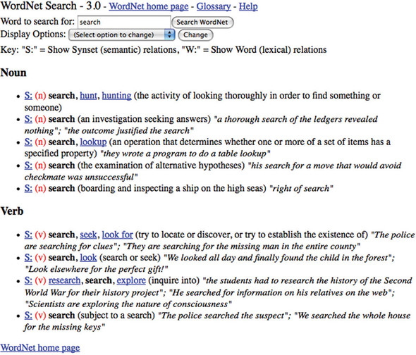
What does all this mean to developers using Lucene? With Dave Spencer’s contribution to Lucene’s contrib modules, the WordNet synonym database can be churned into a Lucene index. This allows for rapid synonym lookup—for example, for synonym injection during indexing or querying (see section 4.5 for such an implementation). We first see how to build an index containing WordNet’s synonyms, then how to use these synonyms during analysis.

9.3.1. Building the synonym index

To build the synonym index, follow these steps:

1.  Download and expand the Prolog version of WordNet, currently distributed as the file WNprolog-3.0.tar.gz from the WordNet site at http://wordnet.princeton.edu/wordnet/download.

2.  Obtain the binary (or build from source; see section 8.7) of the contrib WordNet package.

3.  Un-tar the file you downloaded. It should produce a subdirectory, prolog, that has many files. We’re only interested in the wn_s.pl file. Build the synonym index using the Syns2Index program from the command line. The first parameter points to the wn_s.pl file and the second argument specifies the path where the Lucene index will be created:

java org.apache.lucene.wordnet.Syns2Index prolog/wn_s.pl wordnetindex

The Syns2Index program converts the WordNet Prolog synonym database into a standard Lucene index with an indexed field word and unindexed fields syn for each document. WordNet 3.0 produces 44,930 documents, each representing a single word; the index size is approximately 2.9MB, making it compact enough to load as a RAMDirectory for speedy access.

A second utility program in the WordNet contrib module lets you look up synonyms of a word. Here’s a sample lookup of a word near and dear to our hearts:

java org.apache.lucene.wordnet.SynLookup indexes/wordnet search

Synonyms found for "search":
explore
hunt
hunting
look
lookup
research
seek

Figure 9.2 shows these same synonyms graphically using Luke.

Figure 9.2. Viewing the synonyms for search using Luke’s documents tab

To use the synonym index in your applications, borrow the relevant pieces from SynLookup, as shown in listing 9.3.

Listing 9.3. Looking up synonyms from a WordNet-based index

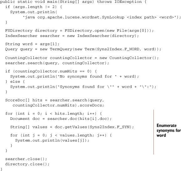
The SynLookup program was written for this book, but it has been added into the WordNet contrib codebase.

9.3.2. Tying WordNet synonyms into an analyzer

The custom SynonymAnalyzer from section 4.5 can easily hook into WordNet synonyms using the SynonymEngine interface. Listing 9.4 contains the WordNetSynonymEngine, which is suitable for use with the SynonymAnalyzer.

Listing 9.4. WordNetSynonymEngine generates synonyms from WordNet’s database

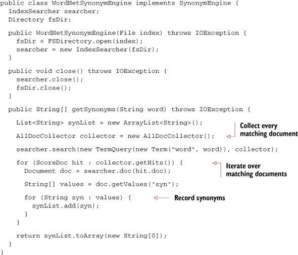
We use the AllDocCollector from section 6.2.3 to keep all synonyms.

Adjusting the SynonymAnalyzerViewer from section 4.5.2 to use the WordNetSynonymEngine, our sample output looks like this:

1: [quick] [warm] [straightaway] [spry] [speedy] [ready] [quickly]
   [promptly] [prompt] [nimble] [immediate] [flying] [fast] [agile]
2: [brown] [embrown] [brownness] [brownish] [browned]
3: [fox][2][trick] [throw] [slyboots] [fuddle] [fob] [dodger]
   [discombobulate] [confuse] [confound] [befuddle] [bedevil]
4: [jumps]
5: [over] [terminated] [o] [ended] [concluded] [complete]
6: [lazy] [slothful] [otiose] [indolent] [faineant]
7: [dogs]

² We’ve apparently befuddled or outfoxed the WordNet synonym database because the synonyms injected for fox don’t relate to the animal noun we intended.

Interestingly, WordNet synonyms do exist for jump and dog, but only in singular form. Perhaps stemming should be added to our SynonymAnalyzer prior to the SynonymFilter, or maybe the WordNetSynonymEngine should be responsible for stemming words before looking them up in the WordNet index. These are issues that need to be addressed based on your environment. This emphasizes again the importance of the analysis process and the fact that it deserves your attention.

We’ll next see some alternative options for holding an index in RAM.

9.4. Fast memory-based indices

In section 2.10 we showed you how to use RAMDirectory to load an index entirely in RAM. This is especially convenient if you have a prebuilt index living on disk and you’d like to slurp the whole thing into RAM for faster searching. But because RAMDirectory still treats all data from the index as files, there’s significant overhead during searching for Lucene to decode this file structure for every query. This is where two interesting contrib modules come in: MemoryIndex and InstantiatedIndex.

MemoryIndex, contributed by Wolfgang Hoschek, is a fast RAM-only index designed to test whether a single document matches a query. It’s only able to index and search a single document. You instantiate the MemoryIndex, then use its addField method to add the document’s fields into it. Then, use its search methods to search with an arbitrary Lucene query. This method returns a float relevance score; 0.0 means there was no match.

InstantiatedIndex, contributed by Karl Wettin, is similar, except it’s able to index and search multiple documents. You first create an InstantiatedIndex, which is analogous to RAMDirectory in that it’s the common store that a writer and reader share. Then, create an InstantiatedIndexWriter to index documents. Alternatively, you can pass an existing IndexReader when creating the InstantiatedIndex, and it will copy the contents of that index. Finally, create an InstantiatedIndexReader, and then an IndexSearcher from that, to run arbitrary Lucene searches.

Under the hood, both of these contributions represent all aspects of a Lucene index using linked in-memory Java data structures, instead of separate index files like RAMDirectory. This makes searching much faster than RAMDirectory, at the expense of more RAM consumption. In many cases, especially if the index is small, the documents you’d like to search have high turnover, the turnaround time after indexing and before searching must be low, and you have plenty of RAM, one of these classes may be a perfect fit.

Next we show how to build queries represented with XML.

9.5. XML QueryParser: Beyond “one box” search interfaces

Contributed by MARK HARWOOD

The standard Lucene QueryParser is ideal for creating the classic single text input search interface provided by web search engines such as Google. But many search applications are more complex than this and require a custom search form to capture criteria with widgets such as the following:

• Drop-down list boxes, such as Gender: Male/Female
• Radio buttons or check boxes, such as Include Fuzzy Matching?
• Calendars for selecting dates or ranges of dates
• Maps for defining locations
• Separate free-text input boxes for targeting various fields, such as title or author

All of the criteria from these HTML form elements must be brought together to form a Lucene search request. There are fundamentally three approaches to constructing this request, as shown in figure 9.3.

Figure 9.3. Three common options for building a Lucene query from a search UI

Options 1 and 2 in figure 9.3 have drawbacks. The standard QueryParser syntax can only be used to instantiate a limited range of Lucene’s available queries and filters. Option 2 embeds all the query logic in Java code, where it can be hard to read or maintain. Generally it’s desirable to avoid using Java code to assemble complex collections of objects. Often a domain-specific text file provides a cleaner syntax and eases maintenance. Further examples include Spring configuration files, XML (Extensible Markup Language) UI (User Interface) Language (XUL) frameworks, Ant build files, or Hibernate database mappings. The contrib XmlQueryParser does exactly this, enabling option 3 from figure 9.3 for Lucene.

We’ll start with a brief example, and then show a full example of how XmlQueryParser is used. We’ll end with options for extending XmlQueryParser with new Query types. Here’s a simple example XML query that combines a Lucene query and filter, enabling you to express a Lucene Query without any Java code:

<FilteredQuery>
  <Query>
    <UserQuery fieldName="text">"Swimming pool"</UserQuery>
  </Query>
  <Filter>
    <TermsFilter fieldName="dayOfWeek">monday friday</TermsFilter>
  </Filter>
</FilteredQuery>

XmlQueryParser parses such XML and produces a Query object for you, and the contrib module includes a full document type definition (DTD) to formally specify the out-of-the-box tags, as well as full HTML documentation, including examples, for all tags.

But how can you produce this XML from a web search UI in the first place? There are various approaches; one simple approach is to use the Extensible Stylesheet Language (XSL) to define query templates as text files that can be populated with user input at runtime. Let’s walk through an example web application. This example is derived from the web demo available in the XmlQueryParser contrib sources.

9.5.1. Using XmlQueryParser

Consider the web-based form UI shown in figure 9.4. Let’s create a servlet that can handle this job search form. The good news is this code should also work, unchanged, with your own choice of form.

Figure 9.4. Advanced search user interface for a job search site, implemented with XmlQueryParser

Our Java servlet begins with some initialization code:

public void init(ServletConfig config) throws ServletException {
  super.init(config);
  try {
    openExampleIndex();

    queryTemplateManager = new QueryTemplateManager(
       getServletContext().getResourceAsStream("/WEB-INF/query.xsl"));

    xmlParser = new CorePlusExtensionsParser(defaultFldName,analyzer);

  } catch (Exception e) {
    throw new ServletException("Error loading query template",e);
  }
}

The initialization code performs three basic operations:

• Opening the search index— Our method (not shown here) simply opens a standard IndexSearcher and caches it in our servlet’s instance data.
• Loading a Query template using the QueryTemplateManager class— This class will be used later to help construct queries.
• Creating an XML query parser— The CorePlusExtensionsParser class used here provides an XML query parser that is preconfigured with support for all the core Lucene queries and filters and also those from Lucene’s contrib modules (we’ll examine how to add support for custom queries later).

Having initialized our servlet, we now add code to handle search requests, shown in listing 9.5.

Listing 9.5. Search request handler using XML query parser

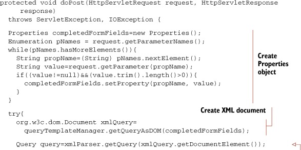
First, a java.util.Properties object is populated with all the form values where the user provided some choice of criteria. If getParameter is used, only one value for a given parameter is allowed; you could switch to getParameterValues instead to relax this limitation. The Properties object is then passed to the QueryTemplateManager to populate the search template and create an XML document that represents our query logic. The XML document is then passed to the query parser to create a Query object for use in searching. The remainder of the method is typical Servlet code used to package results and pass them on to a JavaServer Page (JSP) for display.

Having set up our servlet, we can now take a closer look at the custom query logic we need for our job search and how this is expressed in the query.xsl query template. The XSL language in the query template allows us to perform the following operations:

• Test for the presence of input values with if statements
• Substitute input values in the output XML document
• Manipulate input values, such as splitting strings and zero-padding numbers
• Loop around sections of content using for each statements

We won’t attempt to document all the XSL language here, but clearly the previous list lets us perform the majority of operations that we typically need to transform user input into queries. The XSL statements that control the construction of our query clauses can be differentiated from the query clauses because they’re all prefixed with the <xsl: tag. Our query.xsl is shown in listing 9.6.

Listing 9.6. Using XSL to transform the user’s input into the corresponding XML query

	If the user selects a preference for type of job, apply choice of permanent/contract filter and cache.
	Use standard Lucene query parser for any job description input.
	If any of the location fields are set, OR them all in a Boolean filter and cache individual filters.
	Translate salary range into a constant score range filter.

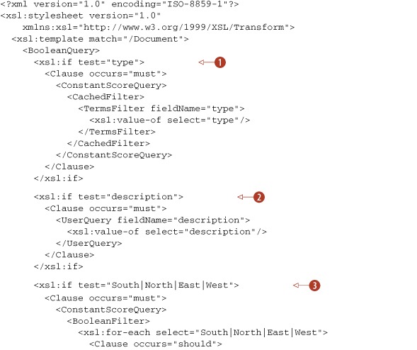
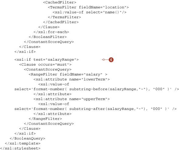
The template in listing 9.6 conditionally outputs clauses depending on the presence of user input. The logic behind each of the clauses is as follows:

• Job type— As a field with only two possible values (permanent or contract), this can be an expensive query clause to run because a search will typically match half of all the documents in our search index. If our index is very large, this can involve reading millions of document IDs from the disk. For this reason we use a cached filter for these search terms. Any filter can be cached in memory for reuse simply by wrapping it in a <CachedFilter> tag.
• Job description— As a free-text field, the standard Lucene query syntax is useful for allowing the user to express his criteria. The contents of the <UserQuery> tag are passed to a standard Lucene QueryParser to interpret the user’s search.
• Job location— Like the job type field, the job location field is a field with a limited choice of values, which benefit from caching as a filter. Unlike the job type field, however, multiple choices of field values can be selected for a location. We use a BooleanFilter to OR multiple filter clauses together.
• Job salary— Job salaries are handled as a RangeFilter clause, which produces a Lucene TermRangeFilter. The input field from the search form requires some manipulation in the XSL template before it can be used. The salary range value arrives from our search form as a single string value such as 90–100. Before we can construct a Lucene request, we must split this into an Upper and Lower value, and make sure both values are zero-padded to comply with Lucene’s requirement for these to be lexicographically ordered. Fortunately these operations can be performed using built-in XSL functions.

Let’s see how to extend XmlQueryParser.

9.5.2. Extending the XML query syntax

Adding support for new tags in the query syntax or changing the classes that support the existing tags is a relatively simple task. As an example, we’ll add support for a new XML tag to simplify the creation of date-based filters. Our new tag allows us to express date ranges in relation to today’s date, such as “last week’s news” or “people aged between 30 and 40.” For example, in our job search application we might want to add a filter using syntax like this:

<Ago fieldName="dateJobPosted" timeUnit="days" from="0" to="7"/>

Each tag in the XML syntax has an associated Builder class, which is used to parse the content. The Builders are registered by adding the object with the name of the tag it supports to the parser. So in order to register a new builder for the Ago tag, we’d need to include a line like the following in the initialization method of our servlet:

xmlParser.addFilterBuilder("Ago", new AgoFilterBuilder());

The AgoFilterBuilder class, shown in listing 9.7, is a simple object that’s used to parse any XML tags with the value Ago. For those familiar with the XML DOM interface, the code should be straightforward.

Listing 9.7. Extending the XML query parser with a custom FilterBuilder

Our AgoFilterBuilder is called by the XML parser every time an Ago tag is encountered, and it’s expected to return a Lucene Filter object given an XML DOM element. The class DOMUtils simplifies the code involved in extracting parameters. Our AgoFilterBuilder reads the to, from, and timeUnit attributes using DOMUtils to provide default values if no attributes are specified. Our code simplifies application logic for specifying to and from values by swapping the values if they’re out of order.

An important consideration in coding Builder classes is that they should be thread-safe. For this reason our class creates a SimpleDateFormat object for each request rather than holding a single object in instance data because SimpleDateFormat isn’t thread-safe.

Our Builder is relatively simple because the XML tag doesn’t permit any child queries or filters to be nested inside it. The BooleanQueryBuilder class in Lucene’s contrib module provides an example of a more complex XML tag that supports nested Query objects. These sorts of Builder classes must be initialized with a QueryBuilderFactory, which is used to find the appropriate Builder to handle each of the nested query tags.

Next we look at an alternate QueryParser that can produce span queries.

9.6. Surround query language

Contributed by PAUL ELSCHOT

As you saw in section 5.5, span queries offer some advanced possibilities for positional matching. Unfortunately, Lucene’s QueryParser is unable to produce span queries. That’s where the Surround QueryParser comes in. The Surround QueryParser defines an advanced textual language to create span queries.

Let’s walk through an example to get a sense of the query language accepted by the Surround QueryParser. Suppose a meteorologist wants to find documents on “temperature inversion.” In the documents, this “inversion” can also be expressed as “negative gradient,” and each word can occur in various inflected forms.

This query in the Surround query language can be used for the “temperature inversion” concept:

5n(temperat*, (invers* or (negativ* 3n gradient*)))

This query will match the following sample texts:

• Even when the temperature is high, its inversion would...
• A negative gradient for the temperature.

But this won’t match the following text, because there’s nothing to match “gradient”:

• A negative temperature.

This shows the power of spans: they allow word combinations in proximity (“negative gradient”) to be treated as synonyms of single words (“inversion”) or of other words in proximity.

You’ll notice the Surround syntax is different from Lucene’s built-in QueryParser. Operators, such as 5n, may be in prefix notation, meaning they come first, followed by their subqueries in parentheses—for example, 5n(...,...). The parentheses for the prefix form gave the name Surround to the language, as they surround the underlying Lucene spans.

The 3n operator is used in infix notation, meaning it’s written between the two subqueries. Either notation is allowed in the Surround query language. The 5n and 3n operators create an unordered SpanNearQuery containing the specified subqueries, meaning they only match when their subqueries have spans within five or three positions of one another. If you replace n with w, then an ordered SpanNearQuery is created. The prefixed number may be from 1 to 99; if you leave off the number (and just type n or w), then the default is 1, meaning the subqueries have adjacent matching spans.

Continuing the example, suppose the meteorologist wants to find documents that match “negative gradient” and two more concepts: “low pressure” and “rain.” In the documents, these concepts can be also expressed in plural or verb form and by synonyms such as “depression” for “low pressure” and “precipitation” for “rain.” Also, all three concepts should occur at most 50 words away from each other:

50n( (low w pressure*) or depression*,
5n(temperat*, (invers* or (negativ* 3n gradient*))),
rain* or precipitat*)

This matches the following sample texts:

• Low pressure, temperature inversion, and rain.
• When the temperature has a negative height gradient above a depression no precipitation is expected.

But it won’t match this text because the word “gradient” is in the wrong place (further than three positions away), leading to improved precision in query results:

• When the temperature has a negative height above a depression no precipitation gradient is expected.

Just like the built-in QueryParser, Surround accepts parentheses to nest queries; field:text syntax to restrict the following search term to a specific field; * and ? as wildcards; Boolean AND, OR, and NOT operators; and the caret (^) for boosting subqueries. When no proximity is used, the Surround QueryParser produces the same Boolean and term queries as the built-in QueryParser. In proximity subqueries, wildcards and or map to SpanOrQuery, and single terms map to SpanTermQuery. Due to limitations of the Lucene spans package, the operators and, not, and ^ can’t be used in subqueries of the proximity operators.

Note that the Lucene spans package is generally not as efficient as the phrase queries used by the standard query parser. And the more complex the query, the higher its execution time. Because of this, we recommend that you provide the user with the possibility of using filters.

Unlike the standard QueryParser, the Surround parser doesn’t use an analyzer. This means that the user will have to know precisely how terms are indexed. For indexing texts to be queried by the Surround language, we recommend that you use a lowercasing analyzer that removes only the most frequently occurring punctuations. Such an analyzer is assumed in the previous examples. Using analyzers this way gives you good control over the query results, at the expense of having to use more wildcards during searching.

With the possibility of nested proximity queries; the need to know precisely what’s indexed; the need to use parentheses, commas, and wildcards; and the preference for additional use of filters, the Surround query language isn’t intended for the casual user. But for those users who are willing to spend more effort on their queries so they can achieve higher-precision results, this query language can be a good fit.

For a more complete description of the Surround query language, have a look at the README.txt file that comes with the source code. To use Surround, make sure that the surround contrib module is on the classpath and follow the example Java code to obtain a normal Lucene query:

String queryText = "5d(temperat*, (invers* or (negativ* 3d gradient*)))";
SrndQuery srndQuery = QueryParser.parse(queryText);
int maxBasicQueries = 1000;

BasicQueryFactory bqFactory = new BasicQueryFactory(maxBasicQueries);

String defaultFieldName = "txt";

Query luceneQuery = srndQuery.makeLuceneQueryField(
             defaultFieldName, bqFactory);

Our next contrib module is called Spatial Lucene.

9.7. Spatial Lucene

Contributed by PATRICK O’LEARY

Over the past decade, web search has transformed itself from finding a basic web page to finding specific results in a certain topic. Video search, medical search, image search, news, sports: each of these is referred to as a vertical search. One that stands out is local search, the use of specialized search techniques that allow users to submit geographically constrained searches against a structured database of local business listings.^[3]

³ Wikipedia provides more details at http://en.wikipedia.org/wiki/Local_search_(Internet).

Lucene now contains a contrib module to enable local search: called Spatial Lucene, it started with the donation of local lucene from Patrick O’Leary (http://www.gissearch.com) and is expected to grow in capabilities over time. If you need to find “shoe stores that exist within 10 miles of location X,” Spatial Lucene will do that.

Though by no means a full GIS (geographical information system) solution, Spatial Lucene supports these functions:

• Radial-based searching; for example, “show me only restaurants within 2 miles from a specified location.” This defines a filter covering a circular area.
• Sorting by distance, so locations closer to a specified origin are sorted first.
• Boosting by distance, so locations closer to a specified origin receive a larger boost.

The real challenge with spatial search is that for every query that arrives, a different origin is required. Life would be simple if the origin were fixed, as we could compute and store all distances in the index. But because distance is a dynamic value, changing with every query as the origin changes, Spatial Lucene must take a dynamic approach that requires special logic during indexing as well as searching. We’ll visit this logic here, as well as touch on some of the performance consideration implied by Spatial Lucene’s approach. Let’s first see how to index documents for spatial search.

9.7.1. Indexing spatial data

To use Spatial Lucene, you must first geo-code locations in your documents. This means a textual location, such as “77 Massachusetts Ave” or “the Louvre” must be translated into its corresponding latitude and longitude. Some methods for geo-coding are described at http://www.gissearch.com/geocode. This process must be done outside of Spatial Lucene, which only operates on locations represented as latitudes and longitudes.

Now what does Spatial Lucene do with each location? One simple approach would be to load each document’s location, compute its distance on the fly, and use that for filtering, sorting, or boosting. This approach will work, but it results in rather poor performance. Instead, Spatial Lucene implements interesting transformations during indexing, including both projection and hierarchical tries and grids, that allow for faster searching.

Projecting the Globe

To compute distances, we first must “flatten” the globe using a mathematical process called projection, depicted in figure 9.5. This is a necessary precursor so that we can represent any location on the surface of the earth using an equivalent two-dimensional coordinate system. This process is similar to having a light shine through a transparent globe and “projected” onto a flat canvas. By unfolding the globe into a flat surface, we make the methods for selecting bounding boxes much more uniform.

Figure 9.5. Projecting the globe’s threedimensional surface into two dimensions is necessary for spatial search.

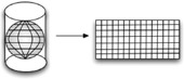
There are two common projections. The first is the sinusoidal projection (http://en.wikipedia.org/wiki/Sinusoidal_projection), which keeps an even spacing of the projection. It will cause a distortion of the image, though, giving it a pinched look. The second projection is the Mercator projection (http://en.wikipedia.org/wiki/Mercator_projection), used because it gives a regular rectangular view of the globe. But it doesn’t correctly scale to certain areas of the planet. If, for example, you look at a global projection of the earth on Google Maps and compare it to the spherical projection in Google Earth, you’ll see that Greenland in Google Maps’ rectangular projection is about the size of North America, whereas in Google Earth, it’s about one third the size. Spatial Lucene has a built-in implementation for the sinusoidal projection, which we’ll use in our example.

The next step is to map each location to a series of grid boxes.

Tiers and Grid Boxes

Once each location is flattened through projection, it’s mapped a hierarchical series of tiers and grid boxes as shown in figure 9.6. Tiers divide the 2D grid into smaller and smaller square grid boxes. Each grid box is assigned a unique ID; as each tier gets higher, the grid boxes become finer.

Figure 9.6. Tiers and grid boxes recursively divide two dimensions into smaller and smaller areas.

This arrangement allows for quick retrieval of locations stored at various levels of granularity. For instance, imagine you have 1 million documents representing different parts of the United States, and you want every document that has a location on the West Coast. If you were storing just the raw document locations, you’d have to iterate through every one of those million documents to see if its location is inside your search radius. But using grids, you can say, “My search radius is about 1,000 miles, so the tier that can best fit a 1,000-mile radius is tier 9, and grid reference –3.004 and –3.005 contain all the items I need.” You then simply retrieve by two terms in Lucene to find the corresponding items. Two term retrievals versus 1 million iterations is a major cost and time savings.

Listing 9.8 shows how to index documents with Spatial Lucene. We use CartesianTierPlotter to create grid boxes for tiers 5 through 15.

Listing 9.8. Indexing a document for spatial search

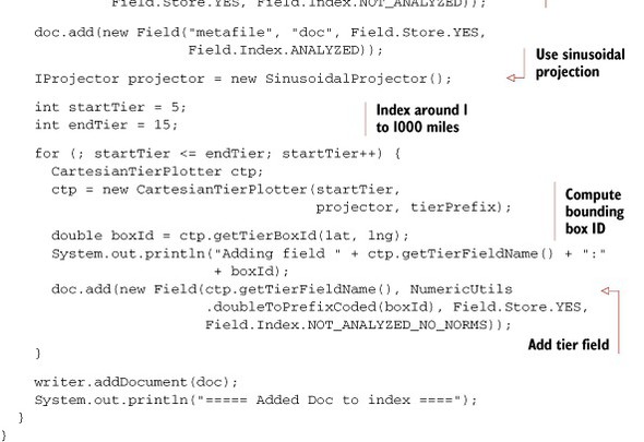
The most important part is the loop that creates the tiers for each location to be indexed. You start by creating a CartesianTierPlotter for the current tier:

ctp = new CartesianTierPlotter(startTier, projector, tierPrefix);

The parameters are as follows:

• tierLevel, in our case starting at 5 and going to 15.
• projector is the SinusoidalProjector, which is the method to project latitude and longitude to a flat surface.
• tierPrefix is the string used as the prefix of the field name, in our case “_localTier”.

We then call ctp.getTierBoxId(lat, lng) with the latitude and longitude values. This returns the ID of the grid box that will contain the latitude and longitude values at this tier level, which is a double representing x,y coordinates. For example, adding field _localTier11:-12.0016 would mean at zoom level 11, box –12.0016 contains the location you’ve added, at grid position x = –12, y = 16. This provides a rapid method for looking up values in an area and finding its nearest neighbors. The method addLocation is simple to use:

addLocation(writer, "TGIFriday", 39.8725000, -77.3829000);

This method will add somewhere called "TGIFriday" with its latitude and longitude coordinates to a Lucene spatial index. Let’s now see how to search the spatial index.

9.7.2. Searching spatial data

Once you have your data indexed, you’ll need to retrieve it; listing 9.9 shows how. We’ll create a method to perform a normal text search that filters and sorts according to distance from a specific origin. This is the basis of a standard local search.

Listing 9.9. Sorting and filtering by spatial criteria

The key component during searching is DistanceQueryBuilder. The parameters are

• latitude and longitude of the center location (origin) for the search
• radius of your search
• latField and lngField, the names of the latitude and longitude fields in the index
• tierPrefix, the prefix of the spatial tiers in the index, which must match the tierPrefix used during indexing
• needPrecise, which is true if you intend to filter precisely by distance

Probably the only parameter whose purpose isn’t obvious is needPrecise. To ensure that all results fit in a radius, the distance from the center location of your search may be calculated for every potential result. Sometimes that precision isn’t needed. For instance, to filter for all locations on the West Coast, which is a fairly arbitrary request, a minimal bounding box could suffice in which case you’d leave needPrecise as false. If you need precisely filtered results, or you intend to sort by distance, you must specify true.

Distance is a dynamic field and not part of the index. That means we must use Spatial Lucene’s DistanceSortSource, which takes the distanceFilter from the DistanceQueryBuilder, because it contains all the distances for the query. Note that the field name (foo, in our example) is unused; DistanceSortSource provides the sorting information. See section 6.1 to learn more about custom sorting. Let’s finish our example.

Finding the Nearest Restaurant

We’ve seen how to populate an index with the necessary information for spatial searching and how to construct a query that filters and sorts by distance. Let’s put the finishing touches on it, combining what we’ve done so far with some spatial data, as shown in listing 9.10. We’ve added an addData method—to enroll a bunch of bars, clubs, and restaurants into the index—along with a main function that creates the index and then does a search for the nearest restaurant.

Listing 9.10. Finding restaurants near home with Spatial Lucene

public static void main(String[] args) throws IOException {
  SpatialLuceneExample spatial = new SpatialLuceneExample();
  spatial.addData();
  spatial.findNear("Restaurant", 39.8725000, -77.3829000, 8);
}

private void addData() throws IOException {
  addLocation(writer, "McCormick & Schmick's Seafood Restaurant",
           39.9579000, -77.3572000);
  addLocation(writer, "Jimmy's Old Town Tavern", 39.9690000, -77.3862000);
  addLocation(writer, "Ned Devine's", 39.9510000, -77.4107000);
  addLocation(writer, "Old Brogue Irish Pub", 39.9955000, -77.2884000);
  addLocation(writer, "Alf Laylah Wa Laylah", 39.8956000, -77.4258000);
  addLocation(writer, "Sully's Restaurant & Supper", 39.9003000, -
     77.4467000);
  addLocation(writer, "TGIFriday", 39.8725000, -77.3829000);
  addLocation(writer, "Potomac Swing Dance Club", 39.9027000, -77.2639000);
  addLocation(writer, "White Tiger Restaurant", 39.9027000, -77.2638000);
  addLocation(writer, "Jammin' Java", 39.9039000, -77.2622000);
  addLocation(writer, "Potomac Swing Dance Club", 39.9027000, -77.2639000);
  addLocation(writer, "WiseAcres Comedy Club", 39.9248000, -77.2344000);
  addLocation(writer, "Glen Echo Spanish Ballroom", 39.9691000, -77.1400000);
  addLocation(writer, "Whitlow's on Wilson", 39.8889000, -77.0926000);
  addLocation(writer, "Iota Club and Cafe", 39.8890000, -77.0923000);
  addLocation(writer, "Hilton Washington Embassy Row", 39.9103000,
           -77.0451000);
  addLocation(writer, "HorseFeathers, Bar & Grill", 39.01220000000001,
           -77.3942);
  writer.close();
}

We add a list of named locations using addData. Then, we search for the word Restaurant in our index within 8 miles from location (39.8725000, –77.3829000). You can run search this by entering ant SpatialLucene at the command prompt. You should see the following result:

Number of results: 3
Found:
Sully's Restaurant & Supper: 3.94 Miles
        (39.9003,-77.4467)
McCormick & Schmick's Seafood Restaurant: 6.07 Miles
        (39.9579,-77.3572)
White Tiger Restaurant: 6.74 Miles
        (39.9027,-77.2638)

As our final topic, let’s look at the performance of Spatial Lucene.

9.7.3. Performance characteristics of Spatial Lucene

Unlike standard text search, which relies heavily on an inverted index where duplication in words reduces the size of an index and improves retrieval time, spatial locations have a tendency to be unique. The introduction of a Cartesian grid with tiers provides the ability to “bucketize” the locations into nonunique grids of different size, thus improving retrieval time. But calculating distance still relies on visiting individual locations in the index. This presents several problems:

• Memory consumption can be high as both the latitude and longitude fields are accessed through the field cache (see section 5.1).
• Results can have varying density.
• Distance calculations are by nature complex and slow.

Memory

Memory can be reduced by using the org.apache.lucene.spatial.geohash methods, which condense the latitude and longitude fields into a single hash field.^[4] The DistanceQueryBuilder supports geohash with its constructor:

⁴ See http://en.wikipedia.org/wiki/Geohash for a good description of what a geohash is.

DistanceQueryBuilder(double lat, double lng, double miles,
                     String geoHashFieldPrefix,
                     String tierFieldPrefix,
                     boolean needPrecise)

There’s a trade-off in the additional processing overhead, though, for encoding and decoding the geohash fields.

Density of Results

As you can imagine, searches for pizza restaurants in Death Valley and New York City will have different characteristics. The more results you have, the more distance calculations you’ll need to perform. Distribution and multithreading help; the more concurrent work you can spread across threads and CPUs, the quicker the response. Caching doesn’t help here, although Spatial Lucene does cache overlapping locations, because the center location of your search may change more frequently than your search term.

 

Note

Don’t index all your data by regions—you’ll find an uneven distribution of load. Cities will generally have more data than suburbs, thus taking more processing time. Furthermore, more people will search for results in cities compared to suburbs.

 

Performance Numbers

As a rough performance test, we evaluated a textual query that filters and sorts by distance. A single thread was used, running on a 3.06 GHz, 1.5 Java virtual machine with a 500MB heap. The searcher was first warmed with 5 queries, and the time averaged five requests for all documents with varying radii. There were 647,860 total documents in the index.

Table 9.1 shows the results. The first column holds the number of documents returned by the query; the second column holds the amount of time for the boundary box calculation, without the precise distance calculation; and the third column indicates the additional time required to get the precise result.

Table 9.1. Searching and filtering time with varying result counts

Number of results	Time to find results	Time to filter by distance
9,959	7 ms	520 ms
14,019	10 ms	807 ms
80,900	12 ms	1,650 ms

It’s clear from table 9.1 that large sets of spatial data can be retrieved from the index rapidly: 12 ms for 80,900 items in a Cartesian boundary box is quite fast. But a significant amount of time is consumed by calculating all the precise result distances to filter out any that might exist outside the radius and to enable sorting.

 

Note

If your main concern is the search score, and a rough bounding box will suffice for precision—for example, all documents in the West Coast compared to all documents precisely within 1,000 miles sorted by distance—then use the DistanceQueryBuilder with needPrecise set to false. You can calculate distances at display time with DistanceUtils.getInstance().getDistanceMi(search_lat, search_long, result_lat, result_lng);.

 

Let’s see a contrib module that enables remote searching using Java’s RMI.

9.8. Searching multiple indexes remotely

The contrib directory includes remote index searching capability through Remote Method Invocation (RMI), under contrib/remote. Although it used to be core functionality inside Lucene, this capability was moved into the contrib area as of the 2.9 release. There are numerous other alternatives to exposing search remotely, such as through web services. This section focuses solely on Lucene’s contrib capabilities; other implementations are left to your innovation.

An RMI server binds to an instance of RemoteSearchable, which is an implementation of the Searchable interface just like IndexSearcher and MultiSearcher. The server-side RemoteSearchable delegates to a concrete Searchable, such as a regular IndexSearcher instance.

Clients to the RemoteSearchable invoke search methods identically to search through an IndexSearcher or MultiSearcher, as shown throughout chapters 3, 5, and 6. Figure 9.7 illustrates one possible remote-searching configuration.

Figure 9.7. Remote searching through RMI, with the server searching multiple indexes

Other configurations are possible, depending on your needs. The client could instantiate a ParallelMultiSearcher over multiple remote (and/or local) indexes, and each server could search only a single index.

To demonstrate RemoteSearchable, we put together a multi-index server configuration, similar to figure 9.7, using both MultiSearcher and ParallelMultiSearcher in order to compare performance. We split the WordNet index (a database of nearly 44,000 words and their synonyms) into 26 indexes representing A through Z, with each word in the index corresponding to its first letter. The server exposes two RMI client-accessible RemoteSearchables, allowing clients to access either the serial MultiSearcher or the ParallelMultiSearcher.

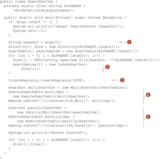
SearchServer is shown in listing 9.11.

Listing 9.11. SearchServer: a remote search server using RMI

	Twenty-six indexes reside under the basedir, each named for a letter of the alphabet.
	A plain IndexSearcher is opened for each index.
	An RMI registry is created.
	A MultiSearcher over all indexes, named LIA_Multi, is created and published through RMI.
	A ParallelMultiSearcher over the same indexes, named LIA_Parallel, is created and published.

Querying through SearchServer remotely involves mostly RMI glue, as shown in SearchClient in listing 9.12. Because our access to the server is through a RemoteSearchable, which is a lower-level API than we want to work with, we wrap it inside a MultiSearcher. Why MultiSearcher? Because it’s a wrapper over Searchables, making it as friendly to use as IndexSearcher.

Listing 9.12. SearchClient accesses RMI-exposed objects from SearchServer

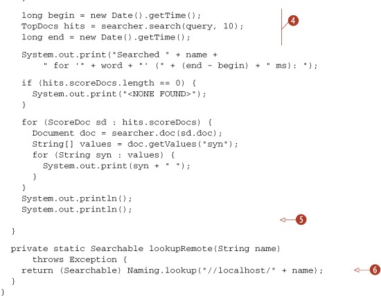
	We perform multiple identical searches to warm up the JVM and get a good sample of response time. The MultiSearcher and ParallelMultiSearcher are each searched.
	The searchers are cached, to be as efficient as possible.
	The remote Searchable is located and wrapped in a MultiSearcher.
	The searching process is timed.
	We don’t close the searcher because it closes the remote searcher, thereby prohibiting future searches.
	Look up the remote interface.

 

Warning

Don’t close() the RemoteSearchable or its wrapping MultiSearcher. Doing so will prevent future searches from working because the server side will have closed its access to the index.

 

Let’s see our remote searcher in action. For demonstration purposes, we ran it on a single machine in separate console windows. The server is started:

% ant SearchServer

Running lia.tools.remote.SearchServer...
Server started
Running lia.tools.remote.SearchClient...
Searched LIA_Multi for 'java' (78 ms): coffee

Searched LIA_Parallel for 'java' (36 ms): coffee

Searched LIA_Multi for 'java' (13 ms): coffee

Searched LIA_Parallel for 'java' (11 ms): coffee

Searched LIA_Multi for 'java' (11 ms): coffee

Searched LIA_Parallel for 'java' (16 ms): coffee

Searched LIA_Multi for 'java' (32 ms): coffee

Searched LIA_Parallel for 'java' (21 ms): coffee

Searched LIA_Multi for 'java' (8 ms): coffee

Searched LIA_Parallel for 'java' (15 ms): coffee

It’s interesting to note the search times reported by each type of server-side searcher. The ParallelMultiSearcher is sometimes slower and sometimes faster than the MultiSearcher in our environment (four CPUs, single disk). Also, you can see the reason why we chose to run the search multiple times: the first search took much longer relative to the successive searches, which is probably due to JVM warmup and OS I/O caching. These results point out that performance testing is tricky business, but it’s necessary in many environments. Because of the strong effect your environment has on performance, we urge you to perform your own tests with your own environment. Performance testing is covered in more detail in section 11.1.

If you choose to expose searching through RMI in this manner, you’ll likely want to create a bit of infrastructure to coordinate and manage issues such as closing an index and how the server deals with index updates (remember, the searcher sees a snapshot of the index and must be reopened to see changes).

Let’s explore yet another alternative for parsing queries, the newly added flexible QueryParser.

9.9. Flexible QueryParser

New in the 2.9 release is a modular alternative to Lucene’s core QueryParser, under contrib/queryparser. This flexible QueryParser was donated to Lucene by IBM, where it’s used in a number of internal products in order to share common query parsing infrastructure even when the supported syntax and query production vary substantially. By the time you read this, it’s possible the core QueryParser will have been replaced with this more flexible one.

So what makes this new parser so flexible? It strongly decouples three phases of producing a Query object from an input String:

1. QueryParser—The incoming String is converted into a tree structured representation, where each Query is represented as a query node. This phase is intentionally kept minimal and hopefully is easily reused across many use cases. It’s meant to be a thin veneer that does the initial rote translation of String into a rich query node tree.
2. QueryNodeProcessor—The query nodes are transformed into other query nodes or have their configuration altered. This phase is meant to do most of the heavy lifting—for example, taking into account what query types are allowed, what their default settings areand so forth.
3. QueryBuilder—This phase translates nodes in the query tree into the final Query instances that Lucene requires for searching. Like QueryParser, this is meant to be a thin veneer whose sole purpose is to render the query nodes into the appropriate Lucene Query objects.

There are two packages within the flexible QueryParser. First is the core framework, located under org.apache.lucene.queryParser.core. This package contains all the infrastructure for implementing the three phases of parsing. The second package contains the StandardQueryParser, located under org.apache.lucene.queryParser.standard, and defines components for each of the three core phases of parsing for that match Lucene’s core QueryParser. The StandardQueryParser is nearly a drop-in for any place that currently uses Lucene’s core QueryParser:

Analyzer analyzer = new StandardAnalyzer(Version.LUCENE_30);
StandardQueryParser parser = new StandardQueryParser(analyzer);
Query q = parser.parse("(agile OR extreme) AND methodology", "subject");
System.out.println("parsed " + q);

Although the new parser is pluggable and modular, it does consist of many more classes than the core QueryParser, which can make initial customization more challenging. Listing 9.13 shows how to customize the flexible QueryParser to reject wildcard and fuzzy queries and produce span queries instead of phrase queries. We made these same changes in section 6.3.2 using the core QueryParser. Whereas the core QueryParser allows you to override one method to customize how each query is created, the flexible query parser requires you to create separate query processor or builder classes.

Listing 9.13. Customizing the flexible query parser

In section 6.3 we were able to override single methods in QueryParser. But with the flexible QueryParser we create either a node processor, as we did to reject fuzzy and wildcard queries, or our own node builder, as we did to create a span query instead of a phrase query. Finally, we subclass StandardQueryParser to install our processors and builders.

In our last section, we’ll cover some odds and ends available in the contrib/miscellaneous package.

9.10. Odds and ends

There are a great many other small packages available in the contrib/miscellaneous package, which we’ll list briefly here:

• IndexSplitter and MultiPassIndexSplitter are two tools for taking an existing index and breaking it into multiple parts. IndexSplitter can only break the index according to its existing segments, but is fast because it does simple file-level copying. MultiPassIndexSplitter can break at arbitrary points (equally by document count), but is slower because it visits documents one at a time and makes multiple passes.
• BalancedSegmentMergePolicy is a custom MergePolicy that tries to avoid creating large segments while also avoiding allowing too many small segments to accumulate in the index. The idea is to prevent enormous merges from occurring, which because they are I/O- and CPU-intensive can affect ongoing search performance in a near-real-time search application. MergePolicy is covered in section 2.13.6.
• TermVectorAccessor enables you to access term vectors from an index even in cases where the document wasn’t indexed with term vectors. You pass in a TermVectorMapper, described in section 5.9.3, that will receive the term vectors. If term vectors were stored in the index, they’re loaded directly and sent to the mapper. If not, the information is regenerated by visiting every term in the index and skipping to the requested document. Note that this regeneration process can be very slow on a large index.
• FieldNormModifier is a standalone tool (defines a static main method) that allows you to recompute all norms in your index according to a specified similarity class. It visits all terms in the inverted index for the field you specify, computing the length in terms of that field for all nondeleted documents, and then uses the provided similarity class to compute and set a new norm for each document. This is useful for fast experimentation of different ways to boost fields according to their length by using a custom Similarity class.
• HighFreqTerms is a standalone tool that opens the index at the directory path you provide, optionally also taking a specific field, and then prints out the top 100 most frequent terms in the index.
• IndexMergeTool is a standalone tool that opens a series of indexes at the paths you provide, merging them together using IndexWriter.addIndexes. The first argument is the directory that all subsequent directories will be merged into.
• SweetSpotSimilarity is an alternative Similarity implementation that provides a plateau of equally good lengths when computing field boost. You have to configure it to see the “sweet spot” typical length of your documents, but this can result in solid improvements to Lucene’s relevance. http://wiki.apache.org/lucene-java/TREC_2007_Million_Queries_Track_IBM_Haifa_Team describes a set of experiments on the Trec 2007 Million Queries Track, including SweetSpotSimilarity, that provided sizable improvements to Lucene’s relevance.
• PrecedenceQueryParser is an alternative QueryParser that tries to handle operator precedence in a more consistent manner.
• AnalyzingQueryParser is an extension to QueryParser that also passes the text for FuzzyQuery, PrefixQuery, TermRangeQuery, and WildcardQuery instances through the analysis process (the core QueryParser doesn’t).
• ComplexPhraseQueryParser is an extension to QueryParser that permits embedding of wildcard and fuzzy queries within a phrase query, such as (john jon jonathan~) peters*.

9.11. Summary

This completes our coverage of all of Lucene’s contrib modules!

Spatial Lucene is a delightful package that allows you to add geographic distance filters and sorting to your search application. ChainedFilter allows you to logically combine multiple filters into one.

We saw three alternative query parsers. XmlQueryParser aims to simplify creation of a rich search user interface by parsing XML into queries. The surround QueryParser enables a rich query language for span queries. The flexible QueryParser is a modular approach that strongly decouples three phases of query parsing and provides a drop-in replacement for the core QueryParser. Fast in-memory indices can be created using either MemoryIndex or InstantiatedIndex, or you can easily store your index in a Berkeley DB directory, giving you all the features of BDB, such as full transactions.

If you end up rolling up your sleeves and creating something new and generally useful, please consider donating it to the Lucene contrib repository or making it available to the Lucene community. We’re all more than grateful for Doug Cutting’s generosity for open sourcing Lucene itself. By also contributing, you benefit from a large number of skilled developers who can help review, debug, and maintain it; and, most important, you can rest easy knowing you have made the world a better place!

In the next chapter we’ll cover the Lucene ports, which provide access to Lucene’s functionality from programming languages and environments other than Java.