Chapter 12. Case study 1: Krugle

Krugle: Searching source code

Contributed by KEN KRUGLER and GRANT GLOUSER

Krugle.org provides an amazing service: it’s a source-code search engine that continuously catalogs 4,000+ open source projects (including Lucene and its sister projects under the Apache Lucene umbrella), enabling you to search the source code itself as well as developers’ comments in the source code control system. A search for lucene turns up matches not only from Lucene’s source code, but from the many open source projects that use Lucene.

Krugle is built with Lucene, but there are some fun challenges that emerge when your documents are primarily source code. For example, a search for deletion policy must match tokens like DeletionPolicy in the source code. Punctuation like = and (, which in any other domain would be quickly discarded during analysis, must instead be carefully preserved so that a search like for(int x=0 produces the expected results. Unlike a natural language where the frequent terms are classified as stop words that are then discarded, Krugle must keep all tokens from the source code.

These unique requirements presented a serious challenge, but as we saw in chapter 4, it’s straightforward to create your own analysis chain with Lucene, and this is exactly what the Krugle team has done. A nice side effect of this process is Krugle’s ability to identify which programming language is in use by each source file; this allows you to restrict searching to a specific language. Krugle also carefully crafts queries to match the tokenization done during analysis, such as controlling the position of each term within a PhraseQuery.

There’s also much to learn about how Krugle handles the administrative aspects of Lucene: it must contend with tremendous scale, in both index size and query rate, yet still provide both searching and indexing on a single computer. You can do this by running dedicated, separate JREs for searching and indexing, carefully assigning separate hard drives for each, and managing the “snapshots” that are flipped between two environments. Krugle’s approach for reducing memory usage during searching is also interesting.

The clever approach the Krugle team uses for self-testing—by randomly picking documents in the index to pass in as searches and asserting that the document is returned in the search results—is a technique most search applications could use to keep the end user’s trust.

Without further ado, let’s go through the intricacies of how Krugle.org uses Lucene to create a high-scale source code search engine.

12.1. Introducing Krugle

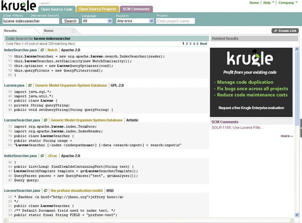
Krugle.org is a search engine for finding and exploring open source projects. The current version has information on the top 4,000+ open source projects, including project descriptions, licenses, SCM activity, and most importantly the source code—more than 400 million lines and growing. Figure 12.1 shows Krugle.org’s search results for the query lucene indexsearcher.

Figure 12.1. The Krugle.org search result page showing matches in multiple projects and multiple source code files

Krugle.org is a free public service, running on a single Krugle enterprise appliance. The appliance is sold to large companies for use inside the firewall. Enterprise development groups use a Krugle appliance to create a single, comprehensive catalog of source code, project metadata, and associated development organization information. This helps them increase code reuse, reduce maintenance costs, improve impact analysis, and monitor development activity across large and often distributed teams.

The most important functionality provided by a Krugle appliance is search, which is based on Lucene. For the majority of users, this means searching through their source code. In this case study we’ll focus on how we used Lucene to solve some interesting and challenging requirements for source code search. Some of these problems often don’t come into play in search applications that involve indexing and searching of human language you find in articles, books, emails, and so forth. But the “tricks” we’ve applied to source code analysis aren’t limited to source code search.

We initially used Nutch to crawl technical web pages, collecting and extracting information about open source projects. We wound up running ten slave servers with one master server in a standard Hadoop configuration, and crawled roughly 50 million pages. The first version of the Krugle.org public site was implemented on top of Nutch, with four remote code searchers, four remote web page searchers, a back-end file server, and one master box that aggregated search results. This scaled easily to 150,000 projects and 2.6 billion lines of source code but wasn’t a suitable architecture for a standalone enterprise product that could run reliably without daily care and feeding. In addition, we didn’t have the commit comment data from the SCM systems that hosted the project source code, which was a highly valuable source of information for both searches and analytics.

So we created a workflow system (internally called “the Hub”) that handled the crawling and processing of data, and converted the original multiserver search system into a single-server solution (“the API”).

12.2. Appliance architecture

For an enterprise search appliance, a challenge is doing two things well at the same time: updating a live index and handling search requests. Both tasks can require extensive CPU, disk, and memory resources, so it’s easy to wind up with resource contention issues that kill your performance.

We made three decisions that helped us avoid these issues. First, we pushed a significant amount of work “off the box” by putting a lot of the heavy lifting work into the hands of small clients called source code management (SCM) interfaces (SCMIs). SCMIs run on external customer servers instead of on our appliance, and act as collectors of information about projects, SCM comments, source code, and other development-oriented information. The information is then partially digested before being sent back to the appliance via a typical HTTP Representational State Transfer (REST) protocol.

Second, we use separate JVMs for the data processing/indexing tasks and the searching/browsing tasks. This provides us with better controlled memory usage, at the cost of some wasted memory. The Hub data processing JVM receives data from the SCMI clients; manages the workflow for parsing, indexing, and analyzing the results; and builds a new “snapshot.” This snapshot is a combination of multiple Lucene indexes, along with all the content and other analysis results. When a new snapshot is ready, a “flip” request is sent to the API JVM that handles the search side of things, and this new snapshot is gracefully swapped in.

On a typical appliance, we have two 32-bit JVMs running, each with 1.5 GB of memory. One other advantage to this approach is that we can shut down and restart each JVM separately, which makes it easier to do live upgrades and debug problems.

Finally, we tune the disks being used to avoid seek contention. There are two drives devoted to snapshots: while one is serving up the current snapshot, the other is being used to build the new snapshot. The Hub also uses two other drives for raw data and processed data, again to allow multiple tasks to run in a multithreaded manner without running into disk thrashing. The end result is an architecture depicted in figure 12.2.

Figure 12.2. Krugle runs two JVMs in a single appliance and indexes content previously collected and digested by external agents.

12.3. Search performance

Due to the specific nature of the domain we’re dealing with (programming languages), we uncovered some interesting areas to optimize. The first issue was the common terms in source code. On the first version of our public site, a search on for (i = 0; i < 10; i++) would bring it to a screeching halt, due to the high frequency of every term in the phrase. But we couldn’t just strip out these common terms (or stop words)—that would prevent phrase queries.

So we borrowed a page from Nutch’s playbook and combined common terms with subsequent terms while indexing and querying using a similar approach as the shingle filter (covered in section 8.2.3). The for loop example results in the combined terms shown in table 12.1.

Table 12.1. Combined terms, which improves performance for common single terms

Term #	Combined Term
1	for (
2	i =
3	0;
4	...
5	++)

The individual terms are still indexed directly, in case you had to search on just i for some bizarre reason. Indexing combined terms results in many more unique terms in the index, but it means that the term frequencies drop—there are a lot fewer documents with 10; than just 10. The resulting list of common terms is shown in table 12.2.

Table 12.2. Most common single and combined terms in the source code index

Single Term	Combined Terms
.	) ;
)	; }
(	( {
;	( )
{	) )
}	} }
=	if (
,	# include
"	; if
>	" )
0	= 0
<	. h
1	( "
/	= =
:	0 ;
-	; return
*	0 )
if	= "
#	{ if
return	# endif
...	...
add	> <

As an example, we have an index for our public site with just under 5 million source files (documents). This results in an index with the attributes shown in table 12.3, for the case where it doesn’t use combined terms versus using 200 combined terms.

Table 12.3. Index file growth after combining high-frequency individual terms

Result	No combined terms	With combined terms
Unique terms	102 million	242 million
Total terms	3.7 billion	13.5 billion
Terms dictionary file size (*.tis)	1.1 GB	2.5 GB
Prox file size (*.prx)	10 GB	18 GB
Freq file size (*.frq)	3.5 GB	7.3 GB
Stored fields file size (*.fdt)	1.0 GB	1.0 GB

We had to switch to a 64-bit JVM and allocate 4 GB of RAM before we achieved reasonable performance with our index.

12.4. Parsing source code

During early beta testing, we learned a lot about how developers search in code, with two features in particular proving to be important. First, we needed to support semistructured searches—for example, where the user wants to limit the search to only find hits in class definition names.

To support this, we had to be able to parse the source code. But “parsing the source code” is a rather vague description. There are lots of compilers that obviously parse source code, but full compilation means that you need to know about include paths (or classpaths), compiler-specific switches, the settings for the macro preprocessor in C/C++, and so forth. The end result is that you effectively need to be able to build the project in order to parse it, and that in turn means you end up with a system that requires constant care and feeding to keep it running. Often that doesn’t happen, so the end result is shelfware.

Early on we made a key decision that we had to be able to process files individually, without knowledge of such things as build settings and compiler versions. We also had to handle a wide range of languages. This in turn meant that the type of parsing we could do was constrained by what features we could extract from a fuzzy parse. We couldn’t build a symbol table, for example, because that would require processing all includes and imports.

Depending on the language, the level of single-file parsing varies widely. Python, Java, and C# are examples of languages where you can generate a good parse tree, whereas C and C++ are at the other end of the spectrum. Dynamic languages like Ruby and Perl create their own unique problems, because the meaning of a term (is it a variable or a function?) sometimes isn’t determined until runtime. So what we wind up with is a best guess, where we’re right most of the time but we’ll occasionally get it wrong.

We use ANTLR (Another Tool for Language Recognition) to handle most of our parsing needs. Terence Parr, the author of ANTLR, added memoization support to version 3.0, which allowed us to use fairly flexible rules without paying a huge performance penalty for frequent backtracking.

12.5. Substring searching

The second important thing we learned from our beta testing was that we had to support some form of substring searching. For example, when a user searches on Idap, she expects to find documents containing terms like getLDAPConfig, IdapTimeout, and find_details_with_ldap.

We could treat every search term as if it had implicit wildcards, like *ldap*, but that’s both noisy and slow. The noise (false positive hits) comes from treating all contiguous runs of characters as potential matches, so a search for heap finds a term like theAPI.

The performance hit comes from having to

• Enumerate all terms in the index to find any that contain <term> as a substring
• Use the resulting set of matching terms in a (potentially very large) OR query BooleanQuery allows a maximum of 1,024 clauses by default—searching on the Lucene mailing list shows many people have encountered this limit while trying to support wildcard queries.

There are a number of approaches to solving the wildcard search problem, some of which we covered in this book. For example, you can take every term and index it using all possible suffix substrings of the text. For example, myLDAPhook gets indexed as myldaphook, yldaphook, ldaphook, and so on. This then lets you turn a search for *ldap* into ldap*, which cuts down on the term enumeration time by being able to do a binary search for terms starting with ldap, rather than enumerating all terms. But you still can end up with a very large number of clauses in the resulting OR query. And the index gets significantly larger, due to term expansion.

Another approach is to convert each term into ngrams—for example, using 3grams the term myLDAPhook would become myl, yld, lda, dap, and so on. Then a search for ldap becomes a search for lda dap in 3grams, which would match. This works as long as N(3, in this example) is greater than or equal to the minimum length of any substring you’d want to find. It also significantly increases the size of the index, and for long terms results in a large number of corresponding ngrams.

Another approach is to preprocess the index, creating a secondary index that maps each distinct substring to the set of all full terms that contain the substring. When a query runs, the first step is to use this secondary index to quickly find all possible terms that contain the query term as a substring, and then use that list to generate the set of subclauses for an OR query. This gives you acceptable query-time speed, at the cost of additional time during index generation. And you’re still faced with potentially exceeding the maximum subclause limit.

We chose a fourth approach, based on the ways identifiers naturally decompose into substrings. We observed that arbitrary substring searches weren’t as important as searches for whole subwords. For example, users expect a search for ldap to find documents containing getLDAPConfig, but it would be unusual for the user to search for apcon with the same expectation.

To implement this approach, we created a token filter that recognizes compound identifiers and splits them up into subwords, a process vaguely similar to stemming (chapter 4 shows how to create custom tokenizers and token filters for analysis). The filter looks for identifiers that follow common conventions like camelCase, or containing numbers or underscores. Some programming languages allow other characters in identifiers, sometimes any character; we stuck with letters, numbers, and underscores as the most common baseline. Other characters are treated as punctuation, so identifiers containing them are still split at those points. The difference is that the next step, subrange enumeration, won’t cross the punctuation boundary.

When we encounter a suitable compound identifier, we examine it to locate the offsets of subword boundaries. For example, getLDAPConfig appears to be composed of the words get, LDAP, and Config, so the boundary offsets are at 0, 3, 7, and 13. Then we produce a term for each pair of offsets (i, j) such that i < j. All terms with a common start offset share a common Lucene index position value; each new start offset gets a position increment of 1.

Table 12.4 shows a table of terms produced for the example getLDAPConfig.

Table 12.4. A case-aware token filter breaks a single token into multiple tokens when the case changes, making it possible to search on subtokens quickly without resorting to more expensive wildcards queries.

Start	End	Position	Term
0	3	1	get
0	7	1	getldap
0	13	1	getldapconfig
3	7	2	Idap
3	13	2	Idapconfig
7	13	3	config

An identifier with n subwords will produce n*(n+1)/2 terms by this method. Because getLDAPConfig has three subwords, we wind up with six terms. By comparison, the number of ngram grows only linearly with the length of the identifier. For example, getLDAPConfig would produce eleven 3grams because it decomposes into get, etl, tld, and so forth. The same level of expansion happens when you generate all suffix substring terms: you end up with getladpconfig, etldapconfig, tldapconfig, and so on until the length of the suffix string reaches your minimum length.

Usually, identifiers consist of at most three or four subwords, so our subrange enumeration produces fewer terms. Pathological cases do exist, resulting in far too many subwords for a given term, so it’s crucial to set some bounds on the enumeration process. Three bounds we set are as follows:

• The maximum length in characters of the initial identifier.
• The maximum number of subwords.
• The maximum span of subwords (k) used to create terms. This limits the number of terms to O(kn).

Because we set the term positions in a nonstandard way while indexing (every compound identifier spans multiple term positions), we also set the term positions in queries. In the simple case, a single identifier, even a compound identifier, becomes a TermQuery. But what about a query that includes punctuation, something like getLDAPConfig()? This becomes a PhraseQuery, where the three terms are getldapconfig, (, and). In the index, getldapconfig spans three term positions, but with a naïve PhraseQuery, Lucene will only match documents in which getldapconfig and a ( are exactly one term position apart. Fortunately, the PhraseQuery API allows you to specify the position of each term using the add(term, position) method, and by counting the span of each term as we add them to the query, we can create a PhraseQuery that exactly matches the position pattern of the desired documents in the index. PhraseQuery is covered in section 3.5.7.

One final snag: occasionally, users are too impatient or lazy to capitalize their queries properly. When the user types getldapconfig() in the search field, we have no basis for calculating how many term positions were supposed to have been spanned by getldapconfig. In lieu of a smarter solution, we deal with this by adding setting the PhraseQuery’s slop (described in section 3.4.6) based on the number and length of such terms.

12.6. Query vs. search

One of the challenges we ran into was the fundamentally different perception of results. In pure search, the user doesn’t know the full set of results and is searching for the most relevant matches. For example, when a user does a search for lucene using Google, he’s looking for useful pages, but he has little to no idea about the exact set of matching pages.

In what we’re calling a query-style search request, the user has more knowledge about the result set and expects to see all hits. He might not look at each hit, but if a hit is missing, the user will typically view this as a bug. For example, when one of our users searches for all callers of a particular function call in their company’s source code, he typically doesn’t know about every single source file where that API is used (otherwise users wouldn’t need us), but users certainly do know of many files that should be part of the result set. And if that “well-known hit” is missing, we’ve got big problems.

So where did we run into this situation? When files are very large, the default setting for Nutch was to only process the first 10,000 terms using Lucene’s field truncation (covered in section 2.7). This in general is okay for web pages but completely fails the query test when dealing with source code. Hell hath no fury like a developer who doesn’t find a large file he knows should be a hit because the search term only exists near the end.

Another example is where we misclassified a file—for example, if file xxx.h was a C++ header instead of a C header. When the user filters search results by programming language, this can exclude files that she knows of and is expecting to see in the result set.

There wasn’t a silver bullet for this problem, but we did manage to catch a lot of problems once we figured out ways to feed our data back on itself. For example, we’d take a large, random selection of source files from the http://www.krugle.org site and generate a list of all possible multiline searches in a variety of sizes (such as 1 to 10 lines). Each search is a small section of source code excised from a random file. We’d then verify that for every one of these code snippets, we got a hit in the original source document.

12.7. Future improvements

As with any project of significant size and complexity, there’s always a long to-do list of future fixes, improvements, and optimizations. A few examples that help illustrate common issues with Lucene follow.

12.7.1. FieldCache memory usage

You know that Lucene’s field cache is memory consuming (see section 5.1), and indeed we noticed on our public site server that more than 1.1 GB was being used by two Lucene field cache data structures. One of these contained the dates for SCM comments, and the other had the MD5 hashes of source files. We need dates to sort commit comments chronologically, and we need MD5s to remove duplicate source files when returning hits. For a thorough explanation about field cache and sorting, see chapter 5.

But a gigabyte is a lot of memory, and this grows to 1.6 GB during a snapshot flip, so we’ve looked into how to reduce the space required. The problems caused by a FieldCache with many unique values is one that’s been discussed on the Lucene list in the past.

For dates, the easy answer is to use longs instead of ISO date strings. The only trick is to ensure that they’re stored as strings with leading zeros so that they still sort in date order. Another option is the use of NumericField, which is described in section 2.6.1.

For MD5s, we did some tests and figured out that using the middle 60 bits of the 128-bit value still provided sufficient uniqueness for 10 million documents. In addition, we could encode 12 bits of data in each character of our string (instead of just 8 bits), so we only need five characters to store the 60 bits, rather than 32 characters for a hex-encoded 128-bit MD5 hash value.

12.7.2. Combining indexes

The major time hit during snapshot creation is merging many Lucene indexes. We cache an up-to-date index for each project, and combine all of these into a single index when generating a snapshot. With over 4,000 projects, this phase of snapshot generation takes almost five hours, or 80 percent of the total snapshot generation time.

Because we have a multicore box, the easiest first cut improvement is to fire off multiple merge tasks (one for each core). The result is many indexes, which we can easily use in the snapshot via a ParallelMultiSearcher (see section 5.8.2). A more sophisticated approach involves segmenting the projects into groups based on update frequency so that a typical snapshot generation doesn’t require merging the project indexes for the projects that are infrequently updated.

12.8. Summary

In 2005 we were faced with a decision about which IR engine to use, and even which programming language made sense for developing Krugle. Luckily we got accurate and valuable input from a number of experienced developers, which answered our two main concerns:

• Java was “fast enough” for industrial-strength search.
• Lucene had both the power and flexibility we needed.

The flexibility of Lucene allowed us to handle atypical situations, such as queries that are actually code snippets or that include punctuation characters that other search engines are typically free to discard. We were also able to handle searches where query terms are substrings of input tokens by using a token filter that’s aware of typical source code naming conventions and thus smart about indexing “compounds” often found in the source code. Without Lucene and the many other open source components we leveraged, there would have been no way to go from zero to beta in six months. So many thanks to our friends for encouraging us to use Lucene, and to the Lucene community for providing such an excellent search toolkit.